Chapter 3. Random Variable and Probability Distribution
🎯 🎲 🎰 🎮
- 3.1 Random Variable
- 3.2 Probability Distribution of Discrete Random Variable
- 3.3 Probability Distribution of Continuous Random Variable
- 3.4 Binomial Distribution
- 3.5 Normal Distribution
- 3.6 Exercise
Probability calculation for certain types of events is widely used in our daily lives. Let's discuss what is a random variable and how to calculate the probability of binomial distribution and normal distribution which are particularly commonly used.
3.1 Random Variable
If there are only two possible outcomes in a trial, it is often observed around us to count the number of one outcome when the trial is repeated several times as follows:
Probabilities can be obtained for various events in the sample space, but what we are more interested in is the events for the number of heads and their probabilities such as tossing a coin two times as follows:
| Event of no head | [TT] | P({TT}) = \(\frac{1}{4}\) |
| Event of one head | {TH, HT} | P({TH, HT}) = \(\frac{2}{4}\) |
| Event of two heads | {HH} | P({HH}) = \(\frac{1}{4}\) |
If \(X\) is the number of heads of the coin, the possible number of \(X\) is 0, 1, and 2. In other words, \(X\) is one-to-one correspondence from each element in the sample space \(S\) to one number as follows:
| Sample space | \(X\) = Number of heads when tossing a coin two times |
|---|---|
| {TT} | 0 |
| {TH} {HT} | 1 |
| {HH | 2 |
The one-to-one relation in which a single real number is matched to each element in the sample space is called the random variable. Random variables are usually denoted with uppercase letters \(X, Y, Z \) ... and values of the random variables are denoted with lowercase letters \(x, y, z \) ... . When a random variable has finite values or countable numbers as a natural number, the random variable is called the discrete random variable, and when it has an arbitrary real value, the random variable is called the continuous random variable. For example, the number of heads that appear by tossing two coins is a discrete random variable, and the delivery time to home when we order a pizza is a continuous random variable because it can have any positive real value.
🎲 Example 3.1
In the next experiments, distinguish whether the random variable \(X\) is a discrete random variable or a continuous random variable.
1) The number of car accidents \(X\) that occur per day at an intersection.
2) The height of our classmates \(X\)
Solution
⏱ Practice 3.1
In the next experiments, distinguish whether the random variable \(X\) is a discrete random variable or a continuous random variable.
1) Number of typhoons \(X\) passing through Korea in a year
2) Annual precipitation \(X\) in Seoul
3) The number of goals\(X\) in a soccer game
4) Height \(X\) of the first-year male high school students
3.2 Probability Distribution of Discrete Random Variable
⭐ Think
When a coin is tossed twice, if \(X\) is the number of heads, the possible values of \(X\) is 0, 1, and 2.💎 Explore
If we arrange all the probabilities for the possible numbers 0, 1, and 2 of \(X\) in a table, what does it look like?
If the random variable \(X\) is the number of heads when a coin is tossed twice, the probability of event which has no head, P({TT}) = \(\frac{1}{4}\), can be written as \(P(X=0) = \frac{1}{4}\). Similarly, the probability of events which has one head, P({TH, HT}) = \(\frac{2}{4}\), as \(P(X=1) = \frac{2}{4}\), and the probability of event which has two heads, P({HH}) = \(\frac{1}{4}\)\(\frac{1}{4}\), as \(P(X=2) = \frac{1}{4}\). These probabilities can be summarized in a table as follows:
| Sample space | \(X\) = Number of heads | \(P(X=x)\) |
|---|---|---|
| {TT} | \(x = 0\) | \(\frac{1}{4}\) |
| {TH} {HT} |
\(x = 1\) | \(\frac{2}{4}\) |
| {HH} | \(x = 2\) | \(\frac{1}{4}\) |
The probability distribution of a discrete random variable \(X\) is a summary of probabilities that \(X\) has a certain value \(x\), \(P(X=x)\), as shown in this table. The above probability distribution can be expressed graphically as in <Figure 3.1>.
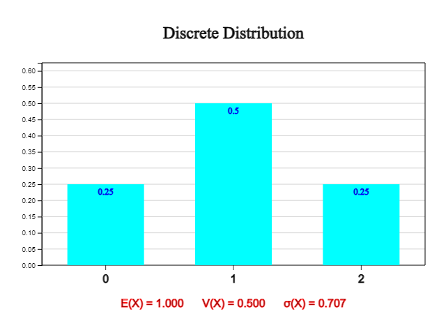
In general, if a discrete random variable \(X\) can have values \(x_1 , x_2 , \cdots , x_n\) and their corresponding probabilities are \(p_1 , p_2 , \cdots , p_n\) respectively, it can be summarized as one-to-one relation as follows and it is called the probability distribution of \(X\).
| \(X\) | \(x_1\) | \(x_2\) | \(\cdots\) | \(x_n\) | Total |
|---|---|---|---|---|---|
| \(P(X=x_i )\) | \(p_1\) | \(p_2\) | \(\cdots\) | \(p_n\) | 1 |
It may also be represented as a mathematical function and it is called the probability density function of \(X\).
Among discrete random variables, the most widely used in reality is the binomial distribution, which will be studied in detail in Section 3.4.
According to the basic properties of probability, the probability distribution function has the following properties.
✨ Properties of probability distribution function
The probability distribution function \(P(X = x_i ) = p_i\) (\(i=1,2, ... , n\)) of a discrete random variable \(X\) has the following properties:
2) \( p_1 + p_2 + \cdots + p_n = 1\)
The probability that a random variable \(X\) has a value between \(a\) and \(b\) is represented as \(P(a \le X \le b)\).
🎲 Example 3.2
There are five products in one box, two of which are defective. We select two products out of this box and inspect them. Let \(X\) be the number of defective items selected.
1) Find the probability distribution of \(X\) and draw a graph using 『eStatH』
2) Find \(P(1 \le X \le 2)\).
Solution
1) \(X\) can have values 0, 1, 2 and their probabilities are as follows:
\(P(X = 1) = \frac{{}_3 C_1 × {}_2 C_1}{{}_5 C_2} = \frac{6}{10}\)
\(P(X = 2) = \frac{{}_3 C_0 × {}_2 C_2}{{}_5 C_2} = \frac{1}{10}\)
Therefore, the probability distribution of \(X\) is represented in a table as follows:
| \(X\) | 0 | 1 | 2 | Total |
|---|---|---|---|---|
| \(P(X=x)\) | \(\frac{3}{10}\) | \(\frac{6}{10}\) | \(\frac{1}{10}\) | 1 |
2) \(P(1 \le X \le 2) = P(X=1) + P(X=2) = \frac{6}{10} + \frac{1}{10} = \frac{7}{10}\)
[Discrete Distribution]
If you select 'Discrete Distribution' from 『eStatH』 menu, data input window such as in <Figure 3.2> appears. Enter the data here as shown in the figure and click [Execute] button to display the probability distribution graph as shown in <Figure 3.3>.
⏱ Practice 3.2
Let a random variable \(X\) be the number of heads when a coin is tossed three times. Find the probability distribution of \(X\) and draw a graph.
A. Mean and standard deviation of a discrete random variable
⭐ Think
If \(X\) = 'the number of heads' when a coin tossed twice, \(X\) can have values 0, 1, and 2 and their probabilities are \(\frac{1}{4}, \frac{2}{4}\) and \( \frac{1}{4}\) respectively.💎 Explore
1) What would be a good representative value of \(X\)?2) What would be a good measure of dispersion for possible values of \(X\)?
The probability distribution of the random variable \(X\) = 'the number of heads' when a coin tossed twice is as follows:
| \(X\) | 0 | 1 | 2 | Total |
|---|---|---|---|---|
| \(P(X=x)\) | \(\frac{1}{4}\) | \(\frac{2}{4}\) | \(\frac{1}{4}\) | 1 |
This probability distribution is similar to the frequency table of three possible values 0, 1, and 2 with the relative frequency.
| Value | Frequency | Relative frequency |
|---|---|---|
| 0 | 1 | \(\frac{1}{4}\) |
| 1 | 2 | \(\frac{2}{4}\) |
| 2 | 1 | \(\frac{1}{4}\) |
| Total | 4 | 1 |
The mean \(\mu\) of these numbers 0, 1, 1, 2 and the variance \(\sigma^2\) are as follows:
Variance \(\;\;\sigma^2 = \frac{(0-1)^2 +(1-1)^2 +(1-1)^2 +(2-1)^2}{4} \)
\(\qquad \qquad \quad \;= (0-1)^2 ×\frac{1}{4} + (1-1)^2 ×\frac{2}{4} + (2-1)^2 ×\frac{1}{4} = \frac{2}{4} = 0.51\)
Therefore, the standard deviation \(\sigma\) is \(\sqrt{0.5} = 0.707 \).
In general, if a discrete random variable \(X\) can have values as \(x_1 , x_2 , \cdots , x_n\) and their probabilities are \(p_1 , p_2 , \cdots , p_n\) respectively, then the probability distribution is as follows
| \(X\) | \(x_1\) | \(x_2\) | \(\cdots\) | \(x_n\) | Total |
|---|---|---|---|---|---|
| \(P(X=x_i )\) | \(p_1\) | \(p_2\) | \(\cdots\) | \(p_n\) | 1 |
The mean or expectation of the random variable \(X\) denoted as \(E(X)\) or \( \mu \), the variance denoted as \(V(X)\) or \(\sigma^2 \) and the standard deviation denoted as \(\sigma(X)\) or \(\sigma\) are calculated as follows:
\(V(X) = \sigma^2 = \sum_{i=1}^{n} (x_i - \mu)^2 p_i\)
\(\sigma(X) = \sqrt{V(X)} \)
The mean or expectation of the random variable \(X\), \(E(X)\), which can have possible values \(x_1 , x_2 , ... , x_n \) with their probabilities \(p_1 , p_2 , ... , p_n \) can be considered as a weighted average of values using the weight of probabilities. The variance of \(X\), \(V(X)\), is a weighted average of all squared distances from the mean. The standard deviation of \(X\), \(\sigma(X)\), is an average distance from the mean.
🎲 Example 3.3
Find the mean, variance and standard deviation of the probability distribution in [Example 3.2]. Check the result using 『eStatH』.
| \(X\) | 0 | 1 | 2 | Total |
|---|---|---|---|---|
| \(P(X=x)\) | \(\frac{3}{10}\) | \(\frac{6}{10}\) | \(\frac{1}{10}\) | 1 |
Solution
The mean, variance and standard deviation of the random variable \(X\) are as follows:
\(V(X) = (0-0.8)^2 ×\frac{3}{10} + (1-0.8)^2 ×\frac{6}{10} + (2-0.8)^2 ×\frac{1}{10} = 0.36\)
\(\sigma(X) = \sqrt{V(X)} = \sqrt{0.36} = 0.6\)
The mean, variance, and standard deviation are consistent with the results of 『eStatH』 in <Figure 3.2>.
⏱ Practice 3.3
When a coin is tossed three times, find the probability distribution by setting the random variable as the number of heads. Find the mean, variance, and standard deviation of this probability distribution.
If we expand the variance of a discrete random variable, \(V(X) = \sigma^2 = \sum_{i=1}^{n} (x_i - \mu)^2 p_i\), it becomes as follows:
\(\qquad\) \(V(X) = (x_{1} - \mu )^{2} p_{1} + (x_{2} - \mu )^{2} p_{2} + \cdots +(x_{n}- \mu )^{2} p_{n} \)
\(\qquad\)\( = (x_{1}^{2} p_{1} -2 \mu x_{1} p_{1} + \mu^{2} p_{i} )+(x_{2}^{2} p_{2} -2 \mu x_{2} p_{2} + \mu^{2} p_{2} )+ \cdots +(x_{n}^{2} p_{2} -2 \mu x_{n} p_{n} + \mu^{2} p_{n} ) \)
\(\qquad\)\( = (x_{1}^{2} p_{1} +x_{2}^{2} p_{2} + \cdots +x_{n} ^{2} p_{n} )-2 \mu (x_{1} p_{1} +x_{2} p_{2} + \cdots +x_{n} p_{n} )+ \mu^{2} (p_{1} +p_{2} + \cdots +p_{n} ) \)
\(\qquad\)\( = E(X^{2} )-2 \mu^{2} + \mu^{2} \)
\(\qquad\)\( = E(X^{2} )- \mu^{2} \)
\(\qquad\)\( = E(X^{2} )-E(X)^{2} \)
Therefore, the variance of a random variable \(X\) can be calculated using a short cut formula as follows:
\(\qquad V(X) = E(X^{2} )-E(X)^{2} \)
Using this short cut formula, the variance of [Example 3.3] can be calculated as follows:
\(\qquad V(X) = (0^{2} × \frac{3}{10} + 1^{2} ×\frac{6}{10} + 2^{2} ×\frac{1}{10} ) - (0.8)^2 = 0.36 \)
✨ Short cut formula of the variance of a discrete random variable \(X\)
If a discrete random variable \(X\) can have values \( x_1 , x_2 , ... , x_n \), their probabilities are \( p_1 , p_2 , ... , p_n \) respectively and \(E(X) = \mu \), then the variance of \(X\) can be calculated as folllows.
\(\quad \quad \;\;= (x_{1}^{2} p_{1} +x_{2}^{2} p_{2} + \cdots +x_{n} ^{2} p_{n} )- \mu^2 \)
🎲 Example 3.4
When a dice is rolled, assume that the number of dots appeared is a random variable \(X\). Find the mean, variance, and standard deviation of \(X\). Draw a graph of the probability distribution using 『eStatH』 and check these values.Solution
The possible values of the random variable \(X\) are 1, 2, 3, 4, 5, 6 and the probability distribution of \(X\) is as follows:
| \(X\) | 1 | 2 | 3 | 4 | 5 | 6 | Total |
|---|---|---|---|---|---|---|---|
| \(P(X=x)\) | \(\frac{1}{6}\) | \(\frac{1}{6}\) | \(\frac{1}{6}\) | \(\frac{1}{6}\) | \(\frac{1}{6}\) | \(\frac{1}{6}\) | 1 |
The mean, variance using a short cut formula and standard deviation are as follows:
\(V(X) = E(X^{2} )-E(X)^{2} = \frac{91}{6} - 3.5^2 = \frac{35}{12} = 2.916\)
\(\sigma(X) = \sqrt{2.916} = 1.708\)
If you select 'Discrete Distribution' from 『eStatH』 menu and enter data as shown in <Figure 3.4>, the graph as shown in <Figure 3.5> and the mean, variance and standard deviation appear. A slightly different value originated from the computing error for the number of decimal places.
[Discrete Distribution]
⏱ Practice 3.4
When a coin is tossed three times, find the probability distribution by setting the random variable \(X\) as the number of heads. Use 『eStatH』 to find the mean, variance, standard deviation and the graph of this probability distribution.
B. Mean and standard deviation of \(a X + b\)
⭐ Think
When a coin tossed twice, the random variable \(X\) = 'number of heads' can have values 0, 1, 2 and their probabilities are \(\frac{1}{4}, \frac{2}{4}, \frac{1}{4}\) respectively.💎 Explore
If \(X\) = 'the number of heads' when a coin is tossed twice, the above game is the same as the problem to examine the probability distribution of 1) \(Y = 100X\) and 2) \(Z = 50 + 100X\). The probability distribution of the random variable \(X\) is as follows and \(E(X)\) = 1, \(V(X)\) = 0.5, \(\sigma(X)\) = 0.707.
| \(X\) | 0 | 1 | 2 | Total |
|---|---|---|---|---|
| \(P(X=x)\) | \(\frac{1}{4}\) | \(\frac{2}{4}\) | \(\frac{1}{4}\) | 1 |
1) The probability distribution of \(Y = 100X\) is as follows:
| \(Y = 100X\) | 0 | 100 | 200 | Total |
|---|---|---|---|---|
| \(P(Y = y)\) | \(\frac{1}{4}\) | \(\frac{2}{4}\) | \(\frac{1}{4}\) | 1 |
Therefore, the expectation \(E(Y)\), variance \(V(Y)\) and standard deviation \(\sigma(Y)\) are as follows:
\(V(Y) = (0-100)^2 ×\frac{1}{4} +(100-100)^2 ×\frac{2}{4} +(200-100)^2 ×\frac{1}{4} = \frac{20000}{4} = 5000 \)
\(\sigma(Y) = \sqrt{5000} = 70.7\)
That is, \(E(Y) = 100 E(X)\), \(V(Y) = 100^2 V(X)\), \(\sigma(Y) = 100 \sigma(X)\).
2) he probability distribution of \(Z = 50 + 100X\) is as follows:
| \(Z = 50 + 100X\) | 50 | 150 | 250 | Total |
|---|---|---|---|---|
| \(P(Y = y)\) | \(\frac{1}{4}\) | \(\frac{2}{4}\) | \(\frac{1}{4}\) | 1 |
Therefore, the expectation \(E(Z)\), variance \(V(Z)\), standard deviation \(\sigma(Z)\) are as follows:
\(V(Z) = (50-150)^2 ×\frac{1}{4} +(150-150)^2 ×\frac{2}{4} +(250-150)^2 ×\frac{1}{4} = \frac{20000}{4} = 5000 \)
\(\sigma(Z) = \sqrt{5000} = 70.7\)
That is, \(E(Z) = 50 + 100 E(X)\), \(V(Z) = 100^2 V(X)\), \(\sigma(Z) = 100 \sigma(X)\).
We noticed that if 50 is added to , the variance of \(Z\) is not affected, but if \(X\) is multiplied by 100, the variance of \(Z\) is increased by \(100^2\).
In general, assume that the probability distribution of a discrete random variable \(X\) is as follows and its mean, variance and standard deviation are \(E(X) = \mu\), \(V(X) = \sigma^2\), \(\sigma(X) = \sigma\) respectively.
| \(X\) | \(x_1\) | \(x_2\) | \(\cdots\) | \(x_n\) | Total |
|---|---|---|---|---|---|
| \(P(X=x )\) | \(p_1\) | \(p_2\) | \(\cdots\) | \(p_n\) | 1 |
The probability distribution of \(Y = aX + b\) is as follows:
| \(Y = aX + b\) | \(y_1 = ax_1 + b\) | \(y_2 = ax_2 + b\) | \(\cdots\) | \(y_n = ax_n + b\) | Total |
|---|---|---|---|---|---|
| \(P(Y=y )\) | \(p_1\) | \(p_2\) | \(\cdots\) | \(p_n\) | 1 |
Therefore, the expectation \(E(Y)\), variance \(V(Y)\) and standard deviation \(\sigma(Y)\) are as follows:
\(\qquad \;= a(x_1 p_1 + x_2 p_2 + \cdots + x_n p_n ) + b(p_1 + p_2 + \cdots +p_n )\)
\(\qquad \;= a E(X) + b = a \mu + b\)
\(V(Y) = [(ax_1 + b) - (a\mu + b)]^2 p_1 + [(ax_2 + b)-(a\mu +b)]^2 p_2 + \cdots + [(ax_n + b)-(a\mu + b)]^2 p_n \)
\(\qquad \;= a^2(x_1 - \mu)^2 p_1 +a^2(x_2 - \mu)^2 p_2 + \cdots + a^2(x_n - \mu)^2 p_n\)
\(\qquad \;= a^2 V(X) = a^2 \sigma^2\)
\(\sigma(Y) = \sqrt{V(Y)} = \sqrt{a^2 \sigma^2} = |a| \sigma \)
If the mean, variance, standardard deviation of a random variable \(X\) are \(E(X) = \mu\), \(V(X) = \sigma^2\), \(\sigma(X) = \sigma\) respectively, then the mean, variance and standard deviation of \(Y = aX + b\) are as follows:
\(V(Y) = a^2 V(X) = a^2 \sigma^2\)
\(\sigma(Y) = \sqrt{a^2 \sigma(X)} = |a| \sigma \)
This is true even if \(X\) is a continuous random variable.
✨ Mean, variance and standard deviation of \(Y = aX + b\)
If \(X\) is a random variable and \( a, b \) are constants, the expectation variance and standard deviation of \(Y = aX + b\) are as follows:
\(V(Y) = a^2 V(X) = a^2 \sigma^2\)
\(\sigma(Y) = \sqrt{a^2 \sigma(X)} = |a| \sigma \)
3.3 Probability Distribution of Continuous Random Variable
⭐ Think
The delivery time to the house by ordering a pizza at a shop were examined 30 times is as follows:
| 15 27 37 9 16 26 17 22 30 23 13 19 22 14 16 18 12 22 16 19 26 11 24 20 21 19 22 11 25 27 |
💎 Explore
Using 『Histogram – Frequency Table』 of 『eStatH』, the histogram of pizza delivery time is as <Figure 3.6> if the class interval starts at 0 and the interval size is 10 minutes. It can be seen that the probability that the pizza is delivered between 10 and 20 minutes is 0.47.
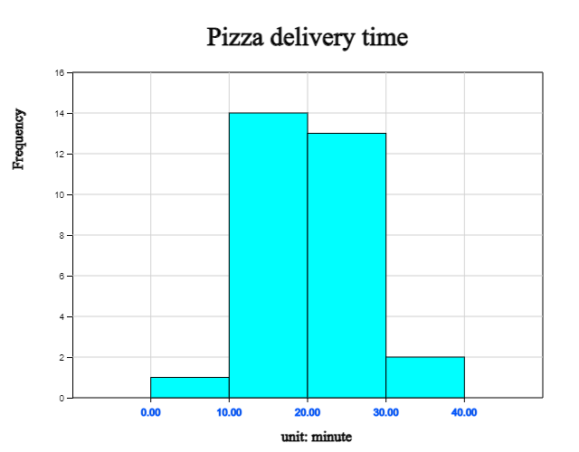
| Class | Frequency | Relative frequency |
|---|---|---|
| 0.00 ≤ x < 10.00 | 1 | 0.03 |
| 10.00 ≤ x < 20.00 | 14 | 0.47 |
| 20.00 ≤ x < 30.00 | 13 | 0.43 |
| 30.00 ≤ x < 40.00 | 2 | 0.07 |
| Total | 30 | 1.00 |
If the interval of the histogram starts at 5 and the interval size is 5 minutes, the histogram becomes as <Figure 3.7>. It can be seen that the probability in which the pizza will be delivered between 15 and 20 minutes is 0.30.
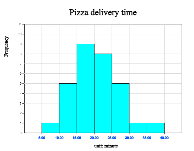
| Class | Frequency | Relative frequency |
|---|---|---|
| 0.00 ≤ x < 5.00 | 1 | 0.03 |
| 10.00 ≤ x < 15.00 | 5 | 0.17 |
| 15.00 ≤ x < 20.00 | 9 | 0.30 |
| 20.00 ≤ x < 25.00 | 8 | 0.27 |
| 25.00 ≤ x < 30.00 | 5 | 0.17 |
| 30.00 ≤ x < 35.00 | 1 | 0.03 |
| 35.00 ≤ x < 40.00 | 1 | 0.03 |
| Total | 30 | 1.00 |
In order to obtain the probability of a more detailed interval, a more detailed histogram such as <Figure 3.8> and its frequency table are required as shown below. However, for such a histogram, more data must be collected, and it is cumbersome to redraw the histogram every time to calculate the desired probability.
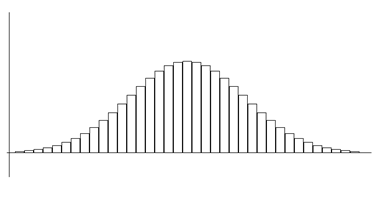
There are many continuous data around us as the histogram above in which many data are located around the mean, data are symmetrical about the mean, and their shape looks like a bell. In order to easily find the probability for all of this type data, mathematicians searched for a function that can describe these kinds of histograms. This function has the same shape as in <Figure 3.9> and is called the normal distribution function. It is explained in detail in Section 3.5.
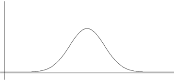
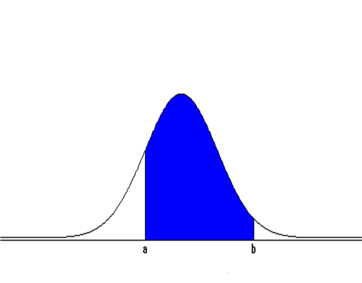
If the probability distribution function of a continuous random variable can be expressed as a mathematical function \(f(x)\), it is possible to approximate the desired probability without finding a frequency table and histogram. In general, the probability distribution function \(f(x)\) of a continuous random variable \(X\) has the following properties.
✨ Properties of the probability distribution function \(f(x)\) of a continuous random variable \(X\).
🎲 Example 3.5
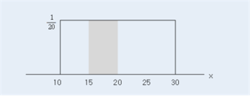
Suppose the delivery time from ordering a pizza to its arrival home can be any time between 10 and 30 minutes. If \(X\) is the random variable of 'delivery time to home', find the probability distribution function of \(X\) and draw its graph. Find the probability that the delivery time is in between 15 and 20 minutes.Solution
Since \(X\) can be any number between 10 and 30, the probability distribution function is as follows: $$ \begin{align} f(x) &= \frac{1}{(30-10)}, 10 \le x \le 30\\ &= 0,\qquad elsewhere \\ \end{align} $$ It is called a uniform distribution and denoted as Uniform(10,30).
The probability of the delivery time in between 15 and 20 minutes is plotted as <Figure 3.11>, so the calculation of the probability (area) is (20-15) × (1/20) = 0.25.
⏱ Practice 3.5
If the probability distribution function of a continuous random variable \(X\) is \(f(x) = 2x, (0 \le x \le 1)\), find the followings.
1) \(P(0 \le X \le \frac{1}{4})\)
2) \(P(\frac{1}{4} \le X \le 1)\)
⏱ Practice 3.6
If the probability distribution function of a continuous random variable \(X\) is \(f(x) = ax, (0 \le x \le 2)\), find the followings. (\(a\) is a constant)
1) constant \(a\)
2) \(P(0 \le X \le \frac{1}{4})\)
3) \(P(\frac{1}{4} \le X \le 1)\)
3.4 Binomial Distribution
⭐ Think
It is said that the defect rate of products produced in one factory is 0.1. Consider a random variable which is the number of defective products when three products are inspected.💎 Explore
What is the probability distribution function of the random variable \(X\)?
When a product is inspected, if it is a good product, we denote it as G, and if it is a defective product, we denote it as B. When three products are inspected, possible events of the sample space, possible values of the random variable \(X\) which is the number of defective products and their probabilities are as follows:
| Sample space | \(X\) = Number of defectives | \(P(X=x)\) |
|---|---|---|
| GGG | 0 | \((0.9)^3\) |
| GGB GBG BGG |
1 | \(3 (0.1)(0.9)^2\) |
| GBB BGB BBG |
2 | \(3 (0.1)^2(0.9)\) |
| BBB | 3 | \( (0.1)^3\) |
When the number of defectives is 0, the number of cases is one which is from \({}_3 C_0\).
When the number of defectives is 1, the number of cases is three which is from \({}_3 C_1\).
When the number of defectives is 2, the number of cases is three which is from \({}_3 C_2\).
When the number of defectives is 3, the number of cases is 1 which is from \({}_3 C_3\).
Therefore the probability distribution function of the random variable \(X\) can be
expressed as follows:
$$
P(X=x) = {}_3 C_x (0.1)^x (0.9)^{3-x} \quad (x=0,1,2,3)
$$
Similar examples as the above problem, which examines the number of defective products by inspecting the product, are observed frequently around us.
\(\qquad\)- Toss a coin five times to count the number of heads.
\(\qquad\)- Count the number of voters in favor of a particular candidate in an election.
Another example can be found at the following instrument as <Figure 3.12>
in science museums. This instrument drops a ball from the top and, if the ball hit a bar,
it may fall to the left (0 point) or to the right (1 point) with a half chance.
Then the ball drops to the next stage bar again and may fall to the left and right
with a half chance. We examine the distribution of scores after the second stage
when 100 balls are dropped.
[Binomial Experiment]
| \(X\) | 0 | 1 | 2 | \(\cdots\) | \(x\) | \(\cdots\) | n | Total |
|---|---|---|---|---|---|---|---|---|
| \(P(X=x)\) | \({}_n C_0 q^n \) | \({}_n C_1 pq^{n-1}\) | \({}_n C_2 p^2 q^{n-2}\) | \(\cdots\) | \({}_n C_x p^x q^{n-x}\) | \(\cdots\) | \({}_n C_n p^n\) | 1 |
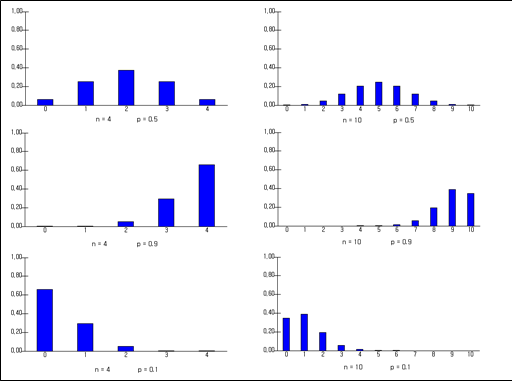
Each probability of this binomial distribution is equal to each coefficient of the terms in the expansion of the equation \((q+p)^n\) using the binomial theorem. $$ (q+p)^n = {}_n C_0 q^n + {}_n C_1 pq^{n-1}+ {}_n C_2 p^2 q^{n-2} + \cdots +{}_n C_x p^x q^{n-x}+ \cdots +{}_n C_n p^n $$ The following is a graph of the binomial distribution for various values of \(n\) and \(p\).
✨ Binomial Distribution
When the Bernoulli trial with probability of 'success' \(p\) is repeated \(n\) times independently, if \(X\) is the random variable of counting the number of 'success', then \(X\) can have values 0, 1, 2, ... , \(n\) and the probability distribution function of \(X\) is a binomial distribution \(B(n,p)\) as follows: $$ f(x) = {}_n C_x p^x (1-p)^{n-x} \quad (x=0,1,2, ... , n) $$
🎲 Example 3.6
In this year baseball season, there are four more games for the team "Tiger" to play with the team "Bear". It is known that 'Tiger' team has a 60% chance of winning every game.
Solution
1) Each game can be considered as a Bernoulli trial of 'Win' or 'Loss' and the trial is repeated four times. If 'Win' is denoted by O and 'Loss' is denoted by X, then there are \(2^4 = 16\) possible elements in the sample space as follows:
S = {'XXXX','OXXX','XOXX','XXOX','XXXO','OOXX','OXOX','OXXO',
'XOOX','XOXO','XXOO','OOOX','OOXO','OXOO','XOOO','XXXX'}
The probability that 'Tiger' will lose four times, {'XXXX'}, is (0.4)×(0.4)×(0.4)×(0.4) = \((0.4)^4\).
The probability that 'Tiger' will lose three times and win one time is
(0.6)×(0.4)×(0.4)×(0.4).
There are four cases of winning one time, {'OXXX', 'XOXX', 'XXOX', 'XXXO'} which are
the same number of cases in which O is seated in one when there are four seats.
So, the probability that 'Tiger' will win once is \({}_4 C_1\). Therefore, the total
probability of winning one game is as follows:
\({}_4 C_1 (0.6)(0.4)^3 \)
The probability that 'Tiger' will lose two times and win also two times is
(0.6)×(0.6)×(0.4)×(0.4).
There are six cases of winning two times,
{'OOXX', 'OXOX', 'OXXO', 'XOOX', 'XOXO', 'XXOO'} which are \({}_4 C_2\).
So the probability of winning two games is as follows:
\({}_4 C_2 (0.6)^2 (0.4)^2 \)
Similarly, the probability of winning three games is as follows:
\({}_4 C_3 (0.6)^3 (0.4) \)
The probability of winning four games is (0.6)×(0.6)×(0.6)×(0.6)
If we summarize, the probability distribution of the random variable \(X\) which is the number of games in which 'Tiger' wins is as follows:
| \(X\) | 0 | 1 | 2 | 3 | 4 | Total |
|---|---|---|---|---|---|---|
| \(P(X=x)\) | \({}_n C_0 (0.4)^4 \) | \({}_n C_1 (0.6)(0.4)^{3}\) | \({}_n C_2 (0.6)^2 (0.4)^{2}\) | \({}_n C_3 (0.6)^3 (0.4)^{1}\) | \({}_n C_4 (0.6)^4 \) | 1 |
2) Select 'Binomial Distribution' from the menu of 『eStatH』 and enter \(n\)= 4, \(p\)= 0.6. If you click [Execute] button, a binomial distribution graph such as <Figure 3.14> appears.
[Binomial Distribution]
There are sliding bars of \(n\) and \(p\) and a probability calculation box under the graph, so put the desired value and press the [Enter] key to calculate the value.
To the right of the graph, a table of binomial distributions is shown. In addition to \(P(X = x)\), this table shows the cumulative probabilities \(P(X \le x)\) and \(P(X \ge x)\) to facilitate various probability calculations. If you select a new \(n\) and \(p\) and click [Execute] button, new binomial distribution table for this value is added below.
⏱ Practice 3.7
The defect rate of an electronic component produced in one factory is 5%. Use 『eStatH』to find the following probabilities when there is a box containing 50 of these components.
1) What's the probability that there is no defective product?
2) What is the probability that there are 1, 2 or 3 defective products?
3) What is the probability of having more than three (≥) defective products?
A. Mean and standard deviation of binomial distribution
If a Bernoulli trial with the probability of 'success' \(p\) and of 'failure' \(q=1-p\) is repeated three times, the random variable \(X\) which counts the number of 'success' is the following binomial distribution.
| \(X\) | 0 | 1 | 2 | 3 | Total |
|---|---|---|---|---|---|
| \(P(X=x)\) | \({}_3 C_0 \;q^3 \) | \({}_3 C_1 \;pq^{2}\) | \({}_3 C_2 \;p^2 q\) | \({}_3 C_3 \;p^3\) | 1 |
The random variable has the mean \(E(X)\), the variance \(V(X)\) and the standard deviation \(\sigma(X)\) as follows:
\(V(X) = (0-3p)^2 ×q^3 + (1-3p)^2 ×3pq^2 + (2-3p)^2 ×3p^2 q + (3-3p)^2 ×p^3 = 3pq\)
\(\sigma(X) = \sqrt{3pq} \)
In general, if a random variable \(X\) follows the binomial distribution, \(B(n,p)\), then its probability distribution is as follows:
| \(X\) | 0 | 1 | 2 | \(\cdots\) | \(x\) | \(\cdots\) | n | Total |
|---|---|---|---|---|---|---|---|---|
| \(P(X=x)\) | \({}_n C_0 q^n \) | \({}_n C_1 pq^{n-1}\) | \({}_n C_2 p^2 q^{n-2}\) | \(\cdots\) | \({}_n C_x p^x q^{n-x}\) | \(\cdots\) | \({}_n C_n p^n\) | 1 |
The mean of \(X\) becomes \(E(X) = np\), the variance becomes \(V(X) = npq\), and the standard deviation becomes \(\sigma(X) = \sqrt{npq}\).
✨ Mean, variance, standard deviation of binomial distribution
If a random variable \(X\) follows binomial \(B(n,p)\),
\(V(X) = npq\)
\(\sigma(X) = \sqrt{npq} \) ( \(q=1-p\))
🎲 Example 3.7
The probability that a salesperson of an insurance company causes a customer to subscribe its insurance is 20% from past experience. A salesperson is scheduled to meet 10 customers this morning. Calculate the following probabilities and use 『eStatH』 to verify them.
1) What is the probability that three customers will subscribe the insurance?
2) What is the probability that two or more people (≥) will subscribe the insurance?
3) On average, how many people will subscribe the insurance? What is its standard deviation?
Solution
It is a binomial distribution with \(n\) = 10 and \(p\) = 0.2.
1) Probability that three customers will subscribe the insurance is as follows:
2) It is better to use the probability of complementary event to calcuate the probability that two or more people (≥) will subscribe the insurance as follows:
\( = 1 - 0.1074 - 0.2684 = 0.6242 \)
3) It is as follows: \(q=1-p\)
\(V(X) = npq = 10 × 0.2 × 0.8 = 1.6 \)
\(\sigma(X) = \sqrt{1.6} = 1.265\)
Select 'Binomial Distribution' in the menu of 『eStatH』 and select \(n\) = 10, \(p\) = 0.2. If you click [Execute] button, the graph as in <Figure 3.16> appears. You can check the probability of 1) if you check the 'probability' here.
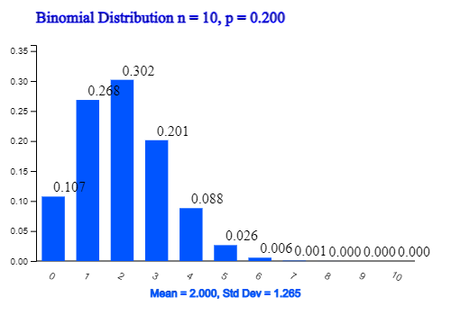
You can check the answer of 2) \(P(X ≥ 2)\) = 0.6242 from the binomial table on the right hand side as follows:
| \(n = 10\) | \(p = 0.200\) | ||
| 0 | 0.1074 | 0.1074 | 1.0000 |
| 1 | 0.2684 | 0.3758 | 0.8926 |
| 2 | 0.3020 | 0.6778 | 0.6242 |
| 3 | 0.2013 | 0.8791 | 0.3222 |
| 4 | 0.0881 | 0.9672 | 0.1209 |
| 5 | 0.0264 | 0.9936 | 0.0328 |
| 6 | 0.0055 | 0.9991 | 0.0064 |
| 7 | 0.0008 | 0.9999 | 0.0009 |
| 8 | 0.0001 | 1.0000 | 0.0001 |
| 9 | 0.0000 | 1.0000 | 0.0000 |
| 10 | 0.0000 | 1.0000 | 0.0000 |
⏱ Practice 3.8
In a presidential election, the approval rating of a particular candidate was 40%. In order to establish an election strategy, we will meet 20 voters this morning to see if they support the particular candidate. Calculate the following probabilities directly and check them using 『eStatH』. Assume that no person abstained.
1) What is the probability that 8 out of 20 will support the particular candidate?
2) What is the probability that 5 or more (≥) and 12 or less (≤) will support?
3) On average, how many people will support the candidate? What's the standard deviation?
If the value of \(n\) is large, it is not easy to calculate the probability of the binomial distribution even using a calculator or computer. In 『eStatH』, you can find the binomial probability when \(n \le 100\). If \(n\) is more than 100, the probability can be approximated using a normal distribution with mean \(np\) and variance \(np(1-p)\). See details in Section 3.5.
B. Law of large number
⭐ Think
Consider an experiment which rolls a dice \(n\) times in which the mathematical probability of each side is \(\frac{1}{6}\). If \(X\) is a random variable which counts the number of single dot on the upper side, \(X\) follows the binomial distribution \(B(n, \frac{1}{6})\).💎 Explore
When you roll a dice \(n\) times, let's compare the relative frequency \(\frac{X}{n}\) with the mathematical probability \(\frac{1}{6}\).
Using the binomial distribution, it can be seen that the mathematical probability of \(\frac{1}{6}\) is a reasonable model. When you roll a dice \(n\) times, the probability that the difference between the relative frequency, \(\frac{X}{n}\), and the mathematical probability, \(\frac{1}{6}\), is less than a small value \(\epsilon\) can be written as follows:
$$ \begin{align} P ( \left | \frac{X}{n} - \frac{1}{6} \right | < \epsilon ) &= P ( \epsilon < \frac{X}{n} - \frac{1}{6} < \epsilon ) \\ &= P ( \frac{1}{6} - \epsilon < \frac{X}{n} < \frac{1}{6} + \epsilon ) \\ &= P \left [ n( \frac{1}{6} - \epsilon )< X < n( \frac{1}{6} + \epsilon ) \right] \end{align} $$ If \(\epsilon\) = 0.1, the above formula becomes as follows: $$ P ( \left | \frac{X}{n} - \frac{1}{6} \right | < 0.1 ) = P \left [ n( \frac{1}{6} - 0.1 ) < X < n( \frac{1}{6} + 0.1 ) \right] $$ If the number of rolls \(n\) is 10, 20, 50, 100, then the above formula becomes as follows and its probability can be calculated using \(B(n, \frac{1}{6})\) in 『eStatH』.
|
\(n = 10\)
\(P \left [ 10( \frac{1}{6} - 0.1 ) < X < 10( \frac{1}{6} + 0.1 ) \right] \) |
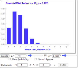
<Figure 3.17> 『eStatH』 \(B(10,0.1667)\)
|
|
\(n = 20\) \(P \left [ 20( \frac{1}{6} - 0.1 ) < X < 20( \frac{1}{6} + 0.1 ) \right] \) \(= P(1.3333 < X < 5.3333) \) \(= P(X=2)+P(X=3)+ P(X=4)+P(X=5) \) \(= 0.7677 \) |
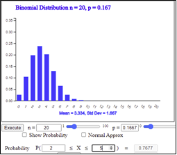
<Figure 3.18> 『eStatH』 \(B(20,0.1667)\)
|
|
\(n = 50\)
\(P \left [ 50( \frac{1}{6} - 0.1 ) < X < 50( \frac{1}{6} + 0.1 ) \right] \) |
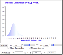
<Figure 3.19> 『eStatH』 \(B(50,0.1667)\)
|
|
\(n = 100\)
\(P \left [ 100( \frac{1}{6} - 0.1 ) < X < 100( \frac{1}{6} + 0.1 ) \right] \) |
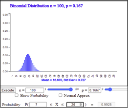
<Figure 3.20> 『eStatH』 \(B(100,0.1667)\)
|
This result is true when \(\epsilon\) is smaller than 0.1 such as 0.01, 0.001, ... which means that the relative frequency \(\frac{X}{n}\) is close to the mathematical probability \(\frac{1}{6}\) if \(n\) is sufficiently large. This is called the law of large number.
✨ Law of large number
Consider a Bernoulli trial with 'success' probability of \(p\) and let a random variable \(X\) be the number of 'success' when the trial is repeated \(n\) times. Ther relative frequency \(\frac{X}{n}\) is close to \(p\) if \(n\) is sufficiently large.
<Figure 3.21> shows that \( P ( \left | \frac{X}{n} - \frac{1}{6} \right | < \epsilon )\) is close to 1 when \(\epsilon\) = 0.05 if \(n\) is increasing up to 1000 by using 『eStatH』. You can change \(p\) and \(\epsilon\) using the slide bars.
3.5 Normal Distribution
⭐ Think
The histogram of delivery times to the house investigated randomly when pizza is ordered are as follows:

💎 Explore
1) What are the characteristics of this histogram?2) What is the mathematical function that can describe this histogram?
Among the data of continuous random variables around us, there are many data which have similar shape such as the histogram above. More data are concentrated near the mean, smaller data are located far from the mean, and data are symmetrical with respect to the mean. In order to find easily the probability of any interval on this shape of data, mathematicians found a function that can describe this shape of data. This mathematical function allows you to approximate the desired probability without finding a frequency table or histogram.
This function was first discovered by Abraham de Moivre (1667-1754), and then widely applied to physics and astronomy by German mathematician Karl Friedrich Gauss (1777-1855). This function is called the normal distribution function or the Gaussian distribution function, and the equation and graph are as follows:
$$ f(x) = \frac{1}{\sqrt{ 2\pi} \sigma } e^{ \left[ - \frac{(x-\mu)^2}{2 \sigma^2} \right]} \qquad - ∞ < x < ∞ $$ where \(\mu\) is a constant, \(\sigma\) is a positive constant, and \(e\) is the irrational number.
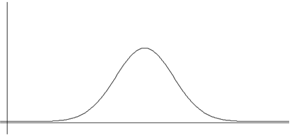
The mean and standard deviation of the normal distribution are \(\mu\) and \(\sigma\) respectively. If a random variable \(X\) follows the normal distribution with the mean \(\mu\) and standard deviation \(\sigma\), that is the variance of \(\sigma^2\), it is denoted as \(N(\mu, \sigma^2 )\).
[ ]
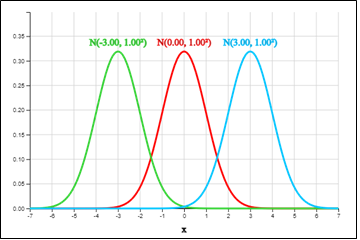
<Figure 3.25> is the graph of three-normal distributions \(N(-3, 1)\), \(N(0, 1)\) and \(N(3, 1)\) in which the mean is different from each other and the variance is all 1. If the mean is different, the graph of the same shape is moved horizontally.
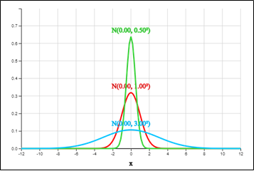
<Figure 3.26> is the graph of three-normal distributions \(N(0, 0.5^2 )\), \(N(0, 1)\) and \(N(0, 3^2 )\) in which all means are zero and variances are different. It can be observed that all of them are symmetrical around the average 0, and that the normal distribution becomes flat as the variance increases, and the normal distribution becomes sharp as the variance decreases.
The characteristics of the normal distribution
A. Probability calculation of Normal distribution
The normal distribution is the most widely used distribution in reality, and it requires a lot of calculation of the probability of the interval \([a, b]\) of the random variable \(X\). As explained earlier, the probability of the interval \([a, b]\), \(P(a \le X \le b)\), when \(X\) follows the normal distribution \(N(\mu, \sigma^2 )\) is the area of the function \(f(x)\) enclosed between the x-axis and interval \([a, b]\)

Mathematically, this area should be obtained as the following definite integral, but it is only possible to use a computer because the function is impossible to integrate. $$ P(a \le X \le b) = \int_a ^b \frac{1}{\sqrt{ 2\pi} \sigma } exp \left[ - \frac{(x-\mu)^2} {2 \sigma^2} \right] dx $$ The probability of the interval \([\mu - \sigma, \mu + \sigma]\) calculated using the computer is 0.68, the probability of the interval \([\mu - 2 \sigma, \mu + 2 \sigma]\) is 0.95, and the probability of the interval \([\mu - 3 \sigma, \mu + 3 \sigma]\) is 0.997. That is, the normal distribution has most values around the mean, and there are few values that are more than three times the standard deviation to the left and right from the mean.
If a random variable \(X\) follows \(N(\mu, \sigma^2 )\), the transformed variable \(Z = \frac{X - \mu}{\sigma}\) follows a normal distribution with mean 0 and standard deviation 1, \(N(0,1)\). This fact implies that if we can find all probabilities of \(N(0,1)\), we can find the probabilities of any normal distribution. Therefore, \(N(0,1)\) is specifically called the standard normal distribution or \(Z\) distribution. The transformation \(Z = \frac{X - \mu}{\sigma}\) that turns a random variable \(X\) into \(Z\) is called the standardized transformation.
✨ Standardized transformation
If a random variable \(X\) follows a normal distribution with with mean \(\mu\) and variance \(\sigma^2\), \(N(\mu, \sigma^2 )\), the transformed variable \(Z = \frac{X - \mu}{\sigma}\) follows a normal distribution with mean 0 and standard deviation 1, \(N(0,1)\). The transformation is called the standardized transformation.
For the standard normal distribution \(N(0,1)\), a table is created by finding the probabilities from the left end to \(z\) for various real values \(z\), \(P(Z \le z)\), which is called the standard normal distribution table. The following table is a part of the standard normal distribution table obtained using 『eStatH』.
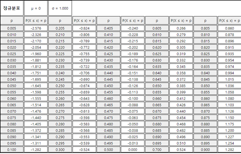
In 『eStatH』, it is easy to calculate the probability for the interval \([a, b]\) of any normal distribution, \(P(a \le X \le b)\), and the percentile \(x\) for a given cumulated probability \(p\), that is \(P(X \le x) = p\), as shown in <Figure 3.28>.
[Normal Distribution]
In 『eStatH』, the probability of an interval can be calculated from \(\mu - 4 \sigma\) to \(\mu + 4 \sigma\). The probability which is less than \(\mu - 4\sigma\) or greater than \(\mu + 4\sigma\) is 0.0000. [Table 3.4] is the percentile table of the standard normal distribution of 『eStatH』.

🎲 Example 3.9
If \(Z\) is the standard normal random variable, find the following probabilities using the standard normal distribution table and confirm it using 『eStatH』.
1) \(P(Z ≤ 1.96)\)
2) \(P(-1.96 ≤ Z ≤ 1.96)\)
3) \(P(Z ≥ 1.96)\)
Solution
When using 『eStatH』 for 1), select the second option under the graph, enter 1.96, and click [Execute] button.
In the same way, 2) is calculated by entering -1.96 and 1.96 in the first option under the graph.
3) is calculated by selecting the third option under the graph and entering 1.96.
🎲 Example 3.10
If \(Z\) is the standard normal random variable, find \(x\) which satisfies the following formula and confirm it using 『eStatH』.
1) \(P(Z ≤ x) = 0.90\)
2) \(P(-x ≤ Z ≤ x) = 0.99\)
3) \(P(Z ≥ x) = 0.05 \)
Solution
When using 『eStatH』 for 1) enter \(p\) = 0.90 in the right box in the fifth option under the graph and click [Execute] button. It can be seen that the correct 90% percentile is 1.282.

For 2) use the fourth option under the graph, enter \(p\) = 0.99 in the right box and click [Execute] button. It can be seen that the correct bilateral percentile are –2.5758 and 2.576.
For 3) use the 6th option under the graph, enter \(p\) = 0.05 in the box on the right and click [Execute] button. It can be seen that the correct right 5% percentile is 1.645.
⏱ Practice 3.9
If \(Z\) is the standard normal random variable, find the following probabilities using the standard normal distribution table and confirm it using 『eStatH』.
1) \(P(-1 ≤ Z ≤ 1)\)
2) \(P(-2 ≤ Z ≤ 2)\)
3) \(P(-3 ≤ Z ≤ 3)\)
⏱ Practice 3.10
If \(Z\) is the standard normal random variable, find \(x\) which satisfies the following formula and cofirm it using 『eStatH』.
1) \(P(Z ≤ x) = 0.99 \)
2) \(P(-x ≤ Z ≤ x) = 0.95 \)
3) \(P(Z ≥ x) = 0.01\)
It is good to remember probabilities of some intervals in the standard normal distribution that are often used. <Figure 3.29> shows the percentiles of 95%, 97.5%, and 99.5% from the left of the standard normal distribution. <Figure 3.30> shows the 95% and 99% probabilities when both ends are equally excluded..
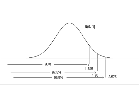
\(\small P(Z \le 1.645) = 0.95, P(Z \le 1.96) = 0.975, P(Z \le 2.575) = 0.995\)
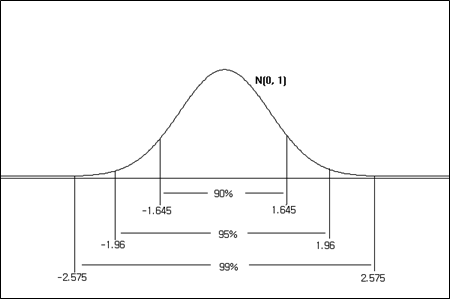
\(\small P(-1.96 \le Z \le 1.96) = 0.95, P(-2.575 \le Z \le 2.575) = 0.99\)
Using the standard normal distribution table, you can find the probability of a general normal distribution. If \(X\) is the normal distribution with mean \(\mu\) and variance \(\sigma^2\), \(\frac{X-\mu}{\sigma}\) follows the standard normal distribution. Therefore, the probability of the interval \([a, b]\) of \(X\), \(P(a \le X \le b)\), is obtained by finding the probability of the interval \([\frac{a-\mu}{\sigma}, \frac{b-\mu}{\sigma}]\) from the standard normal distribution.
✨ Calculation of probability on interval \([a, b]\) in normal distribution
If the random variable \(X\) is the normal distribution with mean \(\mu\) and variance \(\sigma^2\), the probability of the interval \([a, b]\) of \(X\), \(P(a \le X \le b)\) is as follows: $$ P(a \le X \le b) = P(\frac{a-\mu}{\sigma} \le Z \le \frac{b-\mu}{\sigma} ) $$
🎲 Example 3.11
Find the following probability when the midterm score of the Statistics course, \(X\), follows a normal distribution with a mean of 70 point and a standard deviation of 10 points. Check the calculated value using 『eStatH』.
1) \(P(X \le 94.3)\)
2) \(P(X \ge 57.7)\)
3) \(P(57.7 \le X \le 94.3)\)
Solution
The probability calculation of each question is as follows:
\( = 0.8832 \)
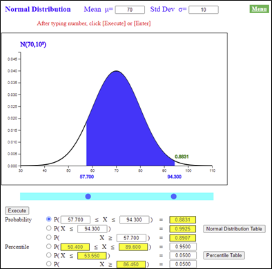
To obtain the probability of a normal distribution using 『eStatH』, first enter the mean as 70 and the standard deviation as 10 on the screen of <Figure 3.31>.
For 1) enter the value of 94.3 in the second option under the graph and click [Execute] button.
In a similar way, for 2) enter 57.7 in the third option to calculate.
For 3) enter the interval as [57.7, 94.3] in the first option and click [Execute] button.
🎲 Example 3.12
Find the following percentiles in [Example 3.11] and confirm the percentiles using 『eStatH』.
1) What is the 95% percentile of the midterm test scores?
2) What is the 95% percentile of excluding the both end sides of the midterm test scores?
Solution
To obtain the percentile of a normal distribution using 『eStatH』, first enter the mean as 70 and the standard deviation as 10 on the screen of <Figure 3.32>.
For 1) enter 0.95 in the right box of the fifth option under the graph and click [Execute] button, the 95% percentile 86.449 appears.
For 2) enter 0.95 in the right box of the fourth option under the graph screen and click [Execute] button to display both 95% percentiles [50.400, 89.600].

⏱ Practice 3.11
It is said that the weight of melons follows a normal distribution with a mean of 250g and a standard deviation of 12g. Find the following probabilities and check the calculation using 『eStatH』.
1) Find the probability that the weight of the melon is less than 260g.
2) Find the probability that the weight of the melon is greater than 240g.
3) Find the probability that the weight of the melon is greater than 240g and less than 260g.
4) Find the weight corresponding to the top 10% of melons.
B. Approximation of Binomial distribution using Normal distribution
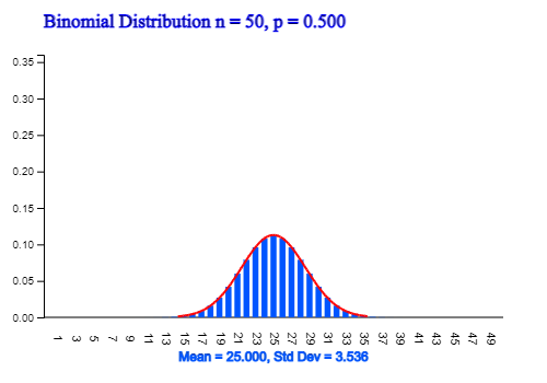
If \(n\) is large (about 50 or more) in case of the binomial distribution, \(B(n,p)\), the probability calculation cannot be obtained even by using 『eStatH』. In this case, the binomial distribution can be approximated using a normal distribution with the mean \(np\), variance \(np(1-p)\). <Figure 3.33> is a graph obtained by approximating the binomial distribution with \(n\) = 50, \(p\) = 0.5 using the normal distribution with the mean \(np=50 \times 0.5 = 25\) and variance \(np=50 \times 0.5 \times 0.5 = 12.5\).
🎲 Example 3.13
It is said that the defective rate of products produced in one factory is 5%. When 100 products were sampled on a day, find the followings.
1) What is the probability that there are less than 2 defective products?
2) What is the probability of 3 to 7 defective products?
Solution
If \(X\) is the number of defective products, then \(X\) is a binomial distribution with \(n\) = 100 and \(p\) = 0.05. In this case, \(n\) is large and the probability can be approximated using the normal distribution. Since the mean of this binomial distribution is \(np\) = 100×0.05 = 5, and the variance is \(np(1-p)\) = 100×0.05×(1-0.05) = 4.75, the probability calculation using the normal distribution \(N(5,4.75)\) is as follows:
1) \(P(X \le 2) = P(Z \le \frac{2-5}{\sqrt {4.75}} ) = P(Z \le 1.376) = 0.0845\)
2) \(P(3 \le X \le 7) = P( \frac{3-5}{\sqrt {4.75}} \le Z \le \frac{7-5}{\sqrt {4.75}} ) = P(-0.918 \le Z \le 0.918) = 0.642\)
⏱ Practice 3.12
In one presidential election, a particular candidate's approval rating was found to be 40%. To develop an election strategy, we will meet with 100 voters today to see if they support the particular candidate. Find the following probability and check it using 『eStatH』. Assume that there is no abstention. 1) What is the probability that 40 or more (≥) and less than (≤) 50 out of 100 voters will support it?2) What is the probability that more than 20 people (≥) will support it?