The quality test for smartphones which may cause a defective or breakage in products cannot be conducted on all products. Therefore, a method of selecting and investigating some of the products produced is usually chosen.

The entire data subject to a statistical survey are called the population, and some of the population selected for the survey are called samples. In general, the population is very large.

In order to find out the characteristic of the population such as the mean, if you survey the entire population, it is called the total survey. However, a total survey of all populations requires enormous costs and time. In addition, a total survey is not appropriate if the product can be destroyed during the inspection such as the impact quality test.

When such a total survey is difficult, the sample survey that investigates some samples from the population is used. Estimating the characteristic of the population using samples selected from the population is called the inferential statistics.

When we estimate the characteristic of the population using samples, the result may vary depending on how samples are selected, so many studies have been conducted on the sampling method. In general, the most commonly used method for sampling is the simple random sampling that ensures that each element in the population has the same probability of being selected. Drawing lots which is often used among friends is an example of a simple random sampling method.

When samples are selected from a population, there are two types of methods such that one is 'with replacement' and the other is 'without replacement'. After a sample is selected, it is included in the population again in case of 'with replacement' method. The selected sample is not included in the population in case of 'without replacement'.

In general, random numbers are used a lot to ensure that each element in the population has the same probability of being selected. Random numbers are numbers that are scattered from 0 to 9 without any particular regularity or bias. [Table 4.1] is a part of the random number table which arranges these random numbers into rows and columns.

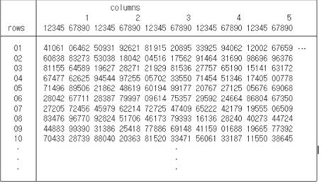
For example, there are 50 students in a class and their identification numbers are 1, 2, ... and 50. In order to select three students of them randomly, first select any one row and one column. If the row 3 and column 11 are selected, read down the double digits starting from here which gives 19, 94, 21, and 28. Among them, numbers outside of 1 to 50 are discarded and three students whose numbers are 19, 21, and 28 are selected.

Simple random sampling using a random number table as shown above is not easy to apply when the sample size is large. Recently random numbers generated by computer using a uniform distribution are commonly used. <Figure 4.1> shows 10 random numbers selected from 1 to 100 numbers without replacement using 『eStatH』.

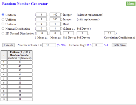
<Figure 4.1> Ten random numbers generated from Uniform(1,100)

By using 『eStatH』, you can also generate random numbers of integer-type Uniform distribution \([a,b]\) with replacement, real-type Uniform distribution \([a,b]\), normal distribution \(N(\mu, \sigma^2 )\), and two-dimensional normal distribution \(N(\mu_1 , \mu_2, \sigma_1 , \sigma_2 , \rho )\).

The purpose of statistical experiments or surveys is to find out the characteristics of the population. The characteristics of the population such as the mean, variance, and standard deviation are called the population mean, population variance and population standard deviation denoted by \(\mu, \sigma^2, \sigma\) respectively.

When \(n\) samples are randomly selected from a population, their mean, variance, and standard deviation are called as the sample mean, sample variance, and sample standard deviation denoted by \(\overline X , S^2 , S\) respectively. If \(X_1 , X_2 , ... , X_n \) represent random variables of samples, \(\overline X , S^2 \) and \(S\) are defined as follows:

In the definition of the sample variance \(S^2\), division by \(n-1\) is to estimate the population variance accurately, but its detail explanation can be done in university level of statistics.

The actual observed values of the random variable \(X_1 , X_2 , ... , X_n \) are denoted as \(x_1 , x_2 , ... , x_n \) and their sample mean, sample variance and sample standard deviation are as follows:

For example, when three samples are taken from the first-year high school male population, the possible number of three samples is countless, so this is indicated as random variables \(X_1 , X_2 , X_3 \). If the actual heights of the three selected students are 160cm, 170cm, and 180cm, these are denoted as \(x_1 = 160, x_2 = 170, x_3 = 180\) and their sample mean, sample variance and sample standard deviations are as follows:

<Figure 4.3> is a simulation that shows the relationship between the characteristic value of the population and the characteristic value of the sample when about 10% of the sample is randomly selected from 10,000 populations of a standard normal distribution using 『eStatH』. Looking at the figure, it can be seen that the minimum (min) and maximum (max) of the population differ from the sample, but there is no significant difference between the population mean and the sample mean.

The population mean, variance and standard deviation are as follows:

The distribution of the population is the unform distribution as follows:

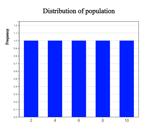
If we select all possible samples of size 2 with replacement and denote two samples as the random variables \(X_1\) and \(X_2\), the sample mean is a random variable \(\overline X = \frac{1}{2} (X_1 + X_2 )\) and a possible value of the sample mean of \(\overline X \) is \(\overline x \). The number of all possible sample means of size 2 with replacement is \(5^2 = 25\) and each sample mean of the samples, \(\overline x \), is as follows:

The frequency table of these 25 sample means and its bar graph are as follows:

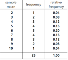
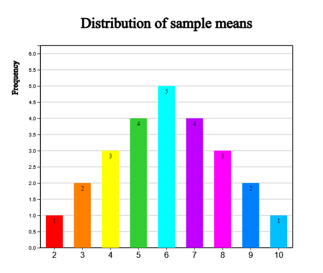
Looking at the frequency table of all possible sample means in [Table 4.3], some of the sample means exactly match the population mean of 6, and others differ greatly, such as 2 or 10. However, looking at <Figure 4.5>, it can be seen that these sample means are concentrated around the population mean of 6.

The average of the 25 sample means in {Table 4.2], \(E(\overline X)\), and variance, \(V(\overline X)\), are as follows:

There are three things that can be observed here.

This relationship between the population mean and all possible sample means is observed even if the population is large or has a different distribution form.

If a population follows the normal distribution of \(N(\mu , \sigma^2 )\), the distribution of all possible samples of size \(n\) which are randomly selected with replacement, the distribution of the sample mean \(\overline X\) follows the normal distribution of \(N(\mu , \frac{\sigma^2}{n} )\). When the distribution of the population does not follow a normal distribution, if the sample size \(n\) is sufficiently large, the distribution of the sample mean \(\overline X\) follows approximately the normal distribution of \(N(\mu , \frac{\sigma^2}{n} )\).

The distribution of the sample mean is very important and it is the fundamental basis of the inferential statistics. <Figure 4.6> is a simulation in 『eStatH』 that shows how the distribution of sample mean varies depending on the size of the sample when the population follows the normal distribution form. Looking at the figure, as the sample size increases, the distribution of the sample mean has the same mean as the population mean, the shape becomes a normal distribution like, and the variance gradually becomes smaller and pointed. This means that if the sample size is very large, the distribution of all possible sample means will be concentrated around the population mean. In other words, the sample mean we obtain is one of all possible sample means, but it is close to the population mean, which is the basis for estimating the population mean well by using any sample mean.

When a sample survey is conducted, only one set of samples is taken from the population to estimate the population mean. In general, we think the mean of the samples as an estimate of the population mean, but can the sample mean obtained from one set of samples among countless possible set of samples predict the population mean well?

The sampling distribution of all possible sample means studied in the previous section is the answer to this question. That is, no matter what a population distribution is, if the sample size is large enough, all possible sample means become dense with a normal distribution shape around the population mean. Therefore, the mean of a set of samples we obtained is usually close to the population mean, and even in the worst case, the difference from the population mean (referred to as an error) is not large, so the sample mean can be said to be a good estimate of the population mean. The larger the sample size, the more dense the distribution of the sample means is, near the population mean, so this error decreases.

The fact that one value of the observed sample mean is an estimate of the population mean is called the point estimation of the population mean (meaning that it is estimated as one number). The sample mean used to estimate the population mean has several good characteristics. One characteristic examined in the previous section is that the mean of all possible sample means becomes to the population mean, and this characteristic is called the unbiased estimate.

Unlike the point estimation, estimating the population mean as an interval is called the interval estimation. If the population is a normal distribution with mean \(\mu\), variance \(\sigma^2\), the distribution of the sample mean \(\overline X\) is the normal distribution with mean \(\mu\) and variance \(\frac{\sigma^2}{n}\), so the probability that one sample mean will be included in the interval \(\mu ± 1.96 \frac{\sigma}{\sqrt{n}}\) is 95% as follows: $$ P ( \mu - 1.96 \frac{\sigma}{\sqrt{n}} \le \overline X \le \mu + 1.96 \frac{\sigma}{\sqrt{n}} ) = 0.95 $$

This equation can also be written as follows: $$ P ( \overline X - 1.96 \frac{\sigma}{\sqrt{n}} \le \mu \le \overline X + 1.96 \frac{\sigma}{\sqrt{n}} ) = 0.95 $$

The meaning of this equation is that 95% of all possible intervals obtained by applying the following interval formula (assuming that \(\sigma\) is known) to all possible sample means include the population mean \(\mu\). The following interval formula is called the 95% confidence interval of the population mean. $$ [ \overline X - 1.96 \frac{\sigma}{\sqrt{n}} , \overline X + 1.96 \frac{\sigma}{\sqrt{n}} ] $$

In general, since \( \overline X ≈ N(\mu , \frac{\sigma^2}{n} )\), the standardized random variable of \(\overline X\), that is \( Z = \frac{\overline X - \mu}{\frac{\sigma}{\sqrt n}} \) follows \( N(0,1) \). Therefore we can write the following probability statement. $$ P ( - z_{\alpha / 2} \le \frac{ \overline X - \mu} {\frac{\sigma}{\sqrt{n}}} \le z_{\alpha /2} ) = 1- \alpha $$

The left hand side of the aboe equation can also be written as follows: $$ P ( \mu - z_{\alpha /2 } \frac{\sigma}{\sqrt{n}} \le \overline X \le \mu + z_{\alpha /2 } \frac{\sigma}{\sqrt{n}} ) = 1- \alpha $$

(1-\(\alpha\)) is called the confidence level, that refers to the probability of intervals in which the population mean is included among all intervals calculated by this interval formula. Usually, 0.01 or 0.05 is used for \(\alpha\). \(z_{\alpha}\) implies a value with a probability at the right end of the standard normal distribution. In other words, if \(Z\) is a random variable that follows the standard normal distribution, the probability that \(Z\) is greater than \(z_{\alpha}\) is \(\alpha\), and if expressed by an equation, \(P(Z \ge z_{\alpha} ) = \alpha \) is established. For example, \(z_{0.025}\) = 1.96, \(z_{0.005}\) = 2.575, etc. Therefore, the 99% confidence interval formula of the population mean is as follows: $$ [ \overline X - 2.575 \frac{\sigma}{\sqrt{n}} , \overline X + 2.575 \frac{\sigma}{\sqrt{n}} ] $$

<Figure 4.7> shows 95% confidence intervals for the population mean by randomly selecting 100 sets of samples with the sample size \(n = 20\) from 10,000 population data which follow the standard normal distribution. In this case, only 94 out of 100 confidence intervals contain the population mean of 0. Whenever these experiments are repeated, results can vary slightly. This simulation shows that, when estimating the confidence interval of the population mean several times, the confidence interval by using the above formula includes the population mean approximately to the confidence level.