Chapter 6. Supervised machine learning for categorical data
CHAPTER OBJECTIVES
The classification analysis technique uses data with known group membership
to create a model to determine the data group with unknown group membership. It has been used in traditional Statistics.
Many new models similar to the classification analysis have been developed to train a computer
for artificial intelligence.
All these models for classification are called models for 'supervised machine learning.'
We introduce the following in this chapter.
• Basic concepts of supervised machine learning and introduce classification analysis models in section 6.1.
• Decision tree model for categorical data in section 6.2.
• General Bayes classification model, a basic statistical classification analysis,
and the naive Bayes classification model for categorical data in section 6.2.
• Evaluation of classification model and comparison methods for several classification models.
6.1 Basic concepts of supervised machine learning and classification
Supervised machine learning is a technique that uses data with known group affiliation to create
a model to determine the group of data whose group affiliation is unknown. It is called as
discriminant analysis or
classification analysis in traditional statistics.
In contrast, a technique that determines groups of similar data using data with unknown group affiliation
is called
cluster analysis or
unsupervised machine learning. A supervised machine learning model
is applied in various fields, such as when a doctor examines a patient and classifies the patient's
diagnosis based on the examination record, when spam mail is filtered out using email subject lines,
and when a customer visiting a department store is identified as a customer who will purchase a product.
A standard method to classify data whose group affiliation is unknown into a group would be
to classify it into the group that is the ‘closest’ to that data.
Many methods define 'closeness' as being from one data source to a group.
For example, the Euclid distance from the data
to the mean of each group, the Minkowski distance, or the Mahalanobis distance,
a statistical measure that considers the variance of the data, can be used. If we consider
a probabilistic approach, there may be a method to estimate the distribution function of each group
and classify data whose group affiliation is unknown into the group it is likely to belong to.
There are many classification models based on various reasonable criteria. In this chapter,
we focus on statistical models for discrete data, such as the decision tree model and the naive Bayes classification model.
Chapter 7 discusses other classification models for continuous data,
such as the k-nearest neighbor model, the neural network model, the support vector machine model, and the ensemble model.
Classification analysis procedure
Assume that there are \(K\) number of groups (or classes) and \(n_1 , n_2 , ... , n_K\) data
were observed in each group. Let \(\boldsymbol x = (x_1 , x_2 , ... , x_m )\) be the observed data of
the random variable \(\boldsymbol X = (X_1 , X_2 , ... , X_m )\). <Figure 6.1.1> shows
the general process of the classification analysis.
Data cleaning and division
Collect data from each group, clean and transform it, and divide the data into training and test data.
|
| ↓ ↑ |
Training the model
Establish a classification model \(y = f( \boldsymbol x ) \) using the training data.
|
| ↓ ↑ |
Validation of the model
Validate the classification model using the testing data.
|
| ↓ |
Apply the model
Classify data whose group affiliation is unknown into one group using the classification model.
|
<Figure 6.1.1> General process of classification analysis
First, data is collected, refined, and transformed appropriately for analysis. Then, the observed data
in each group is divided into training data and testing data. Using the training data, establish
a classification model \(y = f( \boldsymbol x ) \) where \(y\) is the target variable to be estimated,
which means the group. The validity of the model is examined using the testing data.
If this model is not satisfactory, another model is established again, and its validity is examined.
After comparing several classification models and selecting the most satisfactory classification model,
this model is applied to data whose group is unknown to determine which group to classify.
If the variable that represents each group is considered as a dependent variable and the variable
used to classify each group is considered as an independent variable, classification analysis is
similar to regression analysis. However, in regression analysis, the dependent variable is
a random variable that follows a normal distribution, and the levels of the independent variables
are assumed to be given constants, but classification analysis does not make this assumption,
so there is a difference in the model.
Preparation of data for classification analysis
Data for classification analysis should be prepared in advance to improve classification accuracy,
efficiency, and scalability.
A. Data cleaning
If there is noise in the data, it is recommended to remove it. If there are missing values,
it is recommended to preprocess using the corresponding variable's average or mode.
B. Relevance analysis
Among the variables in the data, there may be variables that are not related to classification,
or the variables may be duplicated. Relevance analysis can be used to remove irrelevant or
duplicated variables, improving the classification model's efficiency and accuracy.
C. Data transformation
Continuous data may need to be discretized for classification.
The neural network model requires converting the units of variable values,
such as from -1.0 to 1.0 or from 0.0 to 1.0.
6.1.1 Evaluation measures of classification model
Suppose there are two groups \(\small G_1 , G_2\), and there are \(n\) number of data whose group affiliation is known.
If a classification model is used to classify each data,
the actual group of data and the group classified by the model can be compared and summarized in Table 6.1.1.
| Table 6.1.1 Table for the test results of the actual group and the classified group |
|
|
Classified group |
|
|
|
\(\small G_1\) |
\(\small G_2\) |
Total |
| Actual group |
\(\small G_1\) |
\(\small f_{11}\) |
\(\small f_{12}\) |
\(\small f_{11} + f_{12}\) |
| \(\small G_2\) |
\(\small f_{21}\) |
\(\small f_{22}\) |
\(\small f_{21} + f_{22}\) |
|
Total |
|
|
\(n\) |
Here, \(f_{ij}\) means the number of data of the group \(G_i\) classified into the group \(G_j\).
The number of data correctly classified out of the total data is \(f_{11} + f_{22}\), and the number of data
incorrectly classified is \(f_{12} + f_{21}\). The
accuracy of the classification model
is defined as the ratio of the number of correctly classified data out of the total number of data,
and the
error rate is defined as the ratio of the number of incorrectly classified data
out of the total number of data.
$$
\begin{align}
\text{Accuracy} &= \frac{f_{11} + f_{22}}{n} \\
\text{Error rate} &= \frac{f_{12} + f_{21}}{n}
\end{align}
$$
Generally, classification models strive to find an algorithm that maximizes accuracy or
minimizes error rate. Accuracy and error rate are reasonable criteria assuming that each data
belongs to one group. However, there is a possibility that one data belongs to more than one group,
in which case it is reasonable to predict the probability of belonging to the group.
There are various measures other than accuracy and error rate to evaluate a classification model,
and lift charts, ROC graphs, and statistical analysis methods are used to compare and evaluate various
classification models, which are explained in detail in Section 6.4.
6.1.2 Spliting method for training and testing data
To objectively evaluate a classification model, the entire data set is generally divided
into training data and testing data. The model is established using the training data, and the accuracy
of the model is evaluated using the testing data. If there is sufficient data, validation data is set aside
to improve the performance of the model. This section introduces commonly used methods for dividing
training and testing data.
A. Holdout Method and Random Subsampling
The
holdout method first divides the entire data set into two non-overlapping data sets
and holding out one as training data and the other as testing data. The holdout method is
a widely used method in which a classification model is established using the training data,
and this model is applied to the testing data to measure the accuracy (or error rate).
The ratio at which training and test data are divided depends on the researcher's judgment,
but the most commonly used method is (1/2 training: 1/2 test) or (2/3 training: 1/3 test).
When extracting data at a determined ratio, a simple random sampling method without replacement is used
to reduce bias. The following should be noted when using the reserve method.
1) Since a portion of the entire data for which the group is known is reserved as test data,
there is a risk that the absolute number of training data for establishing the classification model
will be small. In this case, the classification model created with only the training data may not be
as good as the model created using all the data.
2) The classification model may vary depending on how the training and test data are divided.
In general, the smaller the number of training data, the greater the variance in the accuracy of the model.
On the other hand, as the number of training data increases, the reliability of the accuracy estimated
from the test data decreases.
3) Since the training and test data are subsets of the entire data set, they are not independent.
To solve the above problems and to increase the reliability of the accuracy of the classification model,
the preliminary method can be repeatedly performed. Each non-replaced sample is called a subsampling,
and the method of repeatedly extracting them is called the random subsampling method. If the accuracy of
the classification model by the \(i^{th}\) subsampling is \( (Accuracy)_i\), and this experiment is repeated
\(r\) times, the overall accuracy of the classification model is defined as the average of each accuracy
as follows;
$$
\text{Overall accuarcy} = \frac{1}{r} \Sigma_{i=1}^r (Accuracy)_i
$$
Since the random subsampling method does not use the entire data set, just like the holdout method,
it still has problems. However, since the accuracy of the model is repeatedly estimated,
the reliability can be increased.
B. Cross Validation Method
The
cross-validation method is a method that attempts to solve the problems of random subsampling.
Like the holdout method, the entire data set is first divided into training data and testing data.
We create a model using the training data and record the number of data correctly classified by the model
using testing data. Then, the roles of testing data and training data are swapped, and the number of
correctly classified data is added up. It is called the
two-fold cross-validation method, and the accuracy
of the model is calculated as the number of data correctly classified in the entire data. The experiment
is repeated \(r\) times in the same way to obtain the average accuracy. In this method, each data is used once
for training and again for testing, which can somewhat solve the problem of random subsampling.
If the two-fold cross-validation method is extended, the \(k\)-fold cross-validation method can be created.
This method divides the entire data set into \(k\) equal-sized subsets, reserves one of the subsets as
testing data, and uses the remaining data as training data to obtain the classification function.
This method is repeated \(k\) times so that each data subset can be used for testing once.
The accuracy of the classification model is the average of the measured accuracies.
In the cross-validation method, a special case where the total number of data is \(k\), that is,
when there is only one testing data, is called the leave-one-out method. This method has the
advantage of maximizing the training data and testing all data without overlapping the test data.
However, since each testing data contains only one data, there is a disadvantage in that the variance
of the estimated accuracy increases, and since the experiment must be repeated as many times as
the number of data, it takes a lot of time.
C. Bootstrap method
The methods described above extract the training data set from the entire data set without replacement,
so there is no identical data in the training and test data. The bootstrap method extracts
the training data with replacement. The data extracted once is not removed from the entire data set,
and the next data is extracted. When the total number of data is \(N\), and the bootstrap method extracts data,
approximately 63.2% of the entire data is extracted as training data. This is because the probability of
each data being extracted as a bootstrap sample is \(1 - (1 - \frac{1}{N})^N\), and this probability
asymptotically converges to \(1 - \frac{1}{e} \)= 0.632 if \(N\) is sufficiently large. Samples not
extracted by the bootstrap method are used as testing data. A classification model is established
using the data set extracted with replacement as training, and this model is applied to the testing data
to investigate the accuracy. The average of the accuracies measured by repeating similar experiments
is used as the model's overall accuracy.
6.2 Decision tree model
Decision tree is a tree-shaped drawing of a classification function consisting of decision rules,
such as <Figure 6.2.1> which classifies whether a customer visiting a computer store
will purchase a computer. Decision trees are widely used because they are easy to understand
in terms of classification methods and easy to explain results.
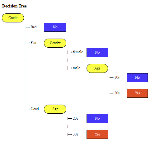
<Figure 6.2.1> A decision tree to classify a customer whether he buys or not
In the tree diagram above, the ovals colored yellow represent
nodes that indicate tests for variables, and the top node
is called the
root node. In <Figure 6.2.1>, Credit is the root node, and Gender and Age are nodes
for testing variables. The
branches from the nodes represent the values of the tested variables,
and the
rectangles colored blue or red represent the final classified groups,
which are called
leaves. The root node, Credit, has three branches 'Bad', 'Fair', and 'Good',
and the classified group for 'Bad' credit is indicated by the leaf 'No' which is the Non-purchasing group.
In order to classify the data whose group is unknown, the variable values of the data are examined
along the path from the root node to the leaves. For example, in <Figure 6.2.1>, a person
whose 'Credit' is 'Good' and 'Age' is '30s' is classified as 'Yes', which is a Purchasing group.
When the target variable is a finite number of groups, such as Purchasing group or Non-purchasing group
in the example above, the tree for classification is called a
decision tree. In the case of
a continuous target variable, we can draw a similar decision tree based on a regression model,
which is called a regression tree (Breiman et al.).
The decision tree model was first attempted by Sonquist and Morgan in 1964 and was widely used
by the general public in 1973 because of Morgan and Messenger's algorithm called THAID. In 1980,
Kass introduced an algorithm called CHAID based on the chi-square goodness-of-fit test,
which is still widely used today. In 1982, computer scientist Quinlan introduced a decision tree algorithm
called ID3 and later developed it into an algorithm called C4.5. In 1984, Breiman et al. established
the theory of decision tree growth and pruning through CART. C4.5 and CART are nonparametric classification methods,
but in 1988, Loh and Vanichetaku introduced FACT, a parametric approach.
Recently, rather than classifying data as a single decision tree, an ensemble model that extracts
multiple samples using the bootstrap method and then integrates multiple decision tree classifications
based on these samples is widely used. The ensemble model is studied in Chapter 7.
6.2.1 Decision tree algorithm
The number of cases for making a decision tree is exponentially proportional to the number of variables
and values for each variable, so there are many cases. Some cases may have higher
classification accuracy than others, and some may have higher accuracy but take too much time.
Therefore, many people have studied to find an answer to the question,
‘How can we find an algorithm that is accurate and has reasonable calculation time?’
A rational algorithm partitions a data set by making locally optimal decisions at each node's decision point
when deciding which variable to use. This method is applied sequentially to the partitioned data sets
to complete a decision tree to partition all data sets. In this section, we introduce an algorithm
as an inductive loop.
[
Decision tree algorithm]: Inductive loop
TreeGrowth (\(\small E, F\))
Step 1: \(\;\;\)if stopping_condition(\(\small E, F\)) = true then
Step 2: \(\qquad\)leaf = creatNode().
Step 3: \(\qquad\)leaf.label = Classify(\(\small E\))
Step 4: \(\qquad\)return leaf
Step 5: \(\;\;\)else
Step 6: \(\qquad\)root = creatNode()
Step 7: \(\qquad\)root.test_condition = find_best_split(\(\small E, F\))
Step 8: \(\qquad\)let \(\small V\) = {\(v: v\) is a possible outcome of root.test_condition}
Step 9: \(\qquad\)for each \(\small v \in V\) do
Step 10: \(\qquad \quad\)\(\small E_v =\){ {root.test_condition(\(\small e\)) = } ∩ {\(\small e \in E\)} }
Step 11: \(\qquad \quad\)child = TreeGrowth(\(\small E_v , F\))
Step 12: \(\qquad \quad\)add child as descendent of root and label the edge(root → child) as \(v\)
Step 13: \(\qquad\)end for
Step 14: \(\;\)end if
Step 15: \(\;\)return root
The algorithm's input is training data \(\small E\) and a variable set \(\small F\).
In step 7 of the algorithm, the optimal variable for splitting the data set is selected (find_best_split),
and in steps 11 and 12, the tree is expanded (TreeGrowth). This process is repeated until the stopping
condition of step 1 is satisfied. The entire algorithm process is explained using an example.
6.2.2 Selection of a variable for branching
In classification using decision trees, deciding which variable to select for each node
is crucial for better classification. Various measures have been studied to choose variables
for optimal branching. A common way to select one variable among several variables would be
to choose a variable that makes classification more accurate for each branch when the variable is selected
and branches out. Let's look at the following example.
Example 6.2.1
In a department store, 20 people who visited a particular store were surveyed, and 8 people (40%) were
in the Purchasing group (\(\small G_1\)) and 12 people (60%) were in the Non-purchasing group (\(\small G_2\)).
The Gender and Credit Status of these 20 people were analyzed and a crosstable was created,
as shown in Table 6.2.1 and Table 6.2.2. Let's find out which variable has better branching in a decision tree.
| Table 6.2.1 Crosstable of Gender by Purchase and Non-purchasing group |
| Gender |
Purchasing group
\(G_1\) |
Non-purchasing group
\(G_2\) |
Total |
| Male |
4 |
6 |
10 |
| Female |
4 |
6 |
10 |
| Total |
8 |
12 |
20 |
| Table 6.2.2 Crosstable of Credit status by Purchase and Non-purchasing group |
| Credit Status |
Purchasing group
\(G_1\) |
Non-purchasing group
\(G_2\) |
Total |
| Good |
7 |
3 |
10 |
| Bad |
1 |
9 |
10 |
| Total |
8 |
12 |
20 |
Answer
In the case of Gender, the ratios of the Purchasing group to the Non-purchasing group for Male and Female are
4 to 6 (40% to 60%), which is the same as the ratio of all 20 people.
In the case of Credit Status, 90% of the customers are in the Non-purchasing group when the Credit Status is Bad,
and 70% are in the Purchasing group when the Credit Status is Good, so there is a significant difference
in the Purchase or Non-purchase ratio between Bad and Good cases. In other words, if the Credit Status
of a customer is Bad, there is a high possibility that he belongs to the Non-purchasing group,
and if it is Good, there is a high possibility that he belongs to the Purchasing group.
So, if the Credit Status is identified, we can distinguish the Purchasing group and the Non-purchasing group can be
somewhat distinguished.
Therefore, if one of the two variables must be selected as a variable for branching
in the decision tree, choosing the Credit Status variable is reasonable for a more accurate classification.
Generally, a variable that has a lot of information for classification is selected.
Many studies have been conducted on how to select a reasonable variable, such as the example above, using
statistical methods. Currently, the most commonly used methods for variable selection in decision trees
include the chi-square independence test, entropy coefficient, Gini coefficient, and classification error rate.
A. Chi-square independence test
The chi-square independence test checks whether the distribution of each group for a variable is independent
or not. In Example 6.2.1, the Gender variable and Purchase status variable can be tested for independence, and
the Credit Status variable and Purchase status variable can be tested for independence.
Suppose there are observed frequencies of a variable \(A\), which are summarized in Table 6.2.3. In that case, the expected frequencies
when the variable \(A\) and the Purchase status variable are independent are calculated in Table 6.2.4.
The expected frequencies are calculated to make the ratios
(\( \frac{O_{\cdot 1}}{O_{\cdot \cdot}} , \frac{O_{\cdot 2}}{O_{\cdot \cdot}}\)) of
the Purchasing group and the Non-purchasing group remain the same in each variable value.
| Table 6.2.3 Observed frequencies of a variable \(A\) by Purchase status group |
Variable \(A\)
value |
Purchasing group
\(G_1\) |
Non-purchasing group
\(G_2\) |
Total |
| \(A_1\) |
\(O_{11}\) |
\(O_{12}\) |
\(O_{1 \cdot}\) |
| \(A_1\) |
\(O_{21}\) |
\(O_{22}\) |
\(O_{2 \cdot}\) |
| Total |
\(O_{\cdot 1}\) |
\(O_{\cdot 2}\) |
\(O_{\cdot \cdot}\) |
| Table 6.2.4 Expected frequencies of a variable by Purchase status when they are independent |
Variable \(A\)
value |
Purchasing group
\(G_1\) |
Non-purchasing group
\(G_2\) |
Total |
| \(A_1\) |
\(E_{11} = O_{1 \cdot} \times \frac{O_{\cdot 1}}{O_{\cdot \cdot}} \) |
\(E_{12} = O_{1 \cdot} \times \frac{O_{\cdot 2}}{O_{\cdot \cdot}}\) |
\(O_{1 \cdot}\) |
| \(A_1\) |
\(E_{21} = O_{2 \cdot} \times \frac{O_{\cdot 1}}{O_{\cdot \cdot}}\) |
\(E_{22} = O_{2 \cdot} \times \frac{O_{\cdot 2}}{O_{\cdot \cdot}}\) |
\(O_{2 \cdot}\) |
| Total |
\(O_{\cdot 1}\) |
\(O_{\cdot 2}\) |
\(O_{\cdot \cdot}\) |
The chi-square statistic of the observed frequencies in Table 6.2.3 for independence test is the sum of
the squares of the differences between the observed and expected frequencies in each cell divided by
the expected frequency.
$$
\chi^2 = \sum_{i=1}^{2} \sum_{j=1}^{2} \frac{ (O_{ij} - E_{ij})^2}{E_{ij}}
$$
This statistic follows the chi-square distribution with a degree of freedom of 1.
Suppose the distribution
of each group in each variable value is the same as the distribution of the entire group. In that case,
the chi-square statistic becomes 0, concluding that the variables and groups are independent.
Suppose the distribution of each group in each variable value is very different from the distribution of
the entire group. In that case, the chi-square statistic becomes very large, and the null hypothesis that the variables
and groups are independent is rejected. The stronger the degree of rejection, the better the variable is
for branching.
Example 6.2.2
Let's examine which variable is better for branching by using the chi-square independence test
for the Gender and Credit Status variable in Example 6.2.1.
Answer
In the crosstable of the Gender and Purchase status, the distribution of
(purchasing group, non-purchasing group) in the entire data is (40%, 60%). The distributions in each Male
and female are also the same at (40%, 60%), so the expected frequencies of Male and Female are (4, 6)
which are the same as observed frequencies and the chi-square statistic \(\chi_{Gender}^2\)is 0 as follows.
$$ \small
\chi_{Credit}^2 = \frac{ (4 - 4)^2}{4} + \frac{ (6 - 6)^2}{6} +\frac{ (4 - 4)^2}{4} +\frac{ (6 - 6)^2}{6} = 0
$$
Therefore, the Gender variable and Purchase status are independent.
In the crosstable of the Credit and Purchase status, the expected frequencies for each Credit status
is (4, 6), so the chi-square statistic is as follows.
$$ \small
\chi_{Credit}^2 = \frac{ (7 - 4)^2}{4} + \frac{ (3 - 6)^2}{6} +\frac{ (1 - 4)^2}{4} +\frac{ (9 - 6)^2}{6} = 7.5
$$
Therefore, since it is greater than the critical value of \(\small \chi_{1;\; 0.05}^2 \) = 3.841 at the significance level of 5%
in the chi-square distribution with the degree of freedom of 1, the Credit variable and Purchase status
are not independent. In other words, if the Credit status is known, it contains a lot of information
to decide the Purchasing group and the Non-purchasing group. Therefore, the branching is selected
by selecting the Credit variable rather than the Gender variable.
If a variable \(A\) has \(a\) number of values and a group variable has \(k\) number of groups,
the chi-square statistic of the \(a \times k\) crosstable is as follows;
$$
\chi^2 = \sum_{i=1}^{a} \sum_{j=1}^{k} \frac{ (O_{ij} - E_{ij})^2}{E_{ij}} \;\;\text{where}\;\; E_{ij} = O_{i \cdot} \times \frac{O_{\cdot j}}{O_{\cdot \cdot}}
$$
This test statistic follows the chi-square distribution with \((a-1)(k-1)\) degree of freedom.
Since the number of values of each variable can be different, the variable with the smaller \(p\)-value
of the chi-square test is used when selecting a variable to split in a decision tree.
B. Entropy coefficient, Gini coefficient, and classification error rate
The entropy coefficient, Gini coefficient, and classification error rate are similar concepts that measure
the uncertainty or purity of a distribution function. If there are \(k\) number of groups,
\(G_1 , G_2 , ... , G_k\), and \(p_1 , p_2 , ... , p_k\) are the probability distribution that
the data belongs to each group, each measure is defined as follows;
$$
\begin{align}
\text{Entropy coefficient} &= - \sum_{i=1}^{k} p_i \times log_{2} p_i \;\; (\text{define}\;\; 0 \times log_{2} 0 = 0 ) \\
\text{Gini coefficient} &= 1 - \sum_{i=1}^{k} p_{i}^2 \\
\text{Classification error rate} &= 1 - max\{p_1 , p_2 , ..., p_k \}
\end{align}
$$
To understand these three measures, let's look at the case where there are only two groups, that is \(k\) = 2.
If the probability of group 1 is \(p\), then the probability of group 2 is \(1-p\). In this case,
the three measures become as follows;
$$
\begin{align}
\text{Entropy coefficient} &= - p \times log_{2} p - (1-p) \times log_{2} (1-p) \\
\text{Gini coefficient} &= 1 - p^2 - (1-p)^2 \\
\text{Classification error rate} &= 1 - max\{p , 1-p \}
\end{align}
$$
<Figure 6.2.2> shows graphs of three measures according to the value of \(p\).
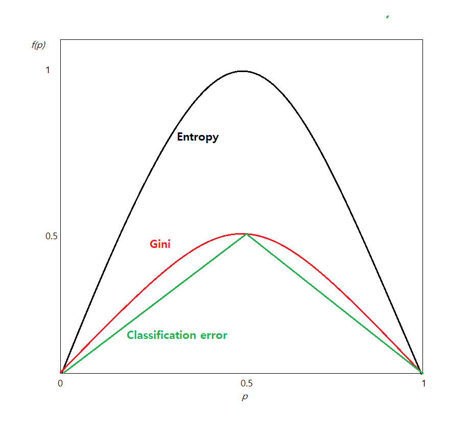
<Figure 6.2.2> Entropy, Gini coefficient, and classification error when there are two groups
As we can see in the figure, all three measures have a maximum value when \(p\) = 0.5 (in this case,
\(1-p\) = 0.5 also, and it is a uniform distribution) and a minimum value of \(p\) = 0 when or \(p\) = 1.
That is, when the probability of two groups is the same (\(p\) = 0.5), uncertainty has a maximum value
because we do not know which group to classify into.
On the other hand, if the probability of one group is 1, there is no uncertainty, that is, the certainty
of classification is 100%, so each measure has a minimum value of 0. Therefore, branching selects a variable
with less uncertainty.
Example 6.2.3
Find the entropy coefficient, Gini coefficient, and classification error rate for the distribution
of the Purchasing group and the Non-purchasing group (40%, 60%) in the entire data. Also, find the
entropy coefficient, Gini coefficient, and classification error rate for each Gender and Credit Status,
and examine which variable is good for branching.
Answer
The entropy coefficient, Gini coefficient, and classification error rate for the probability distribution
(0.4, 0.6) of the Purchasing group and the Non-purchasing group are as in Table 6.2.5, and the measures
for the Gender are in Table 6.2.6, and the measures for the Credit Status are in Table 6.2.7.
| Table 6.2.5 Uncetainty measures for the distribution of (Purchase, Non-purchase) of entire data |
|
Purchasing group
\(G_1\) |
Non-purchasing group
\(G_2\) |
Total |
Uncetainty measures |
Entire data |
8 |
12 |
20 |
$$ \small
\begin{align}
\text{Entropy coefficient} &= - 0.4 \times log_{2} 0.4 - (1-0.4) \times log_{2} (1-0.4) = 0.9710 \\
\text{Gini coefficient} &= 1 - {0.4}^2 - (1-0.4)^2 = 0.4800\\
\text{Classification error rate} &= 1 - max\{0.4 , 1-0.4 \} = 0.4000
\end{align}
$$
|
| Table 6.2.6 Uncetainty measures for the distribution of (Purchase, Non-purchase) of Gender |
| Gender |
Purchasing group
\(G_1\) |
Non-purchasing group
\(G_2\) |
Total |
Uncetainty measures |
Male |
4 |
6 |
10 |
$$ \small
\begin{align}
\text{Entropy coefficient} &= - 0.4 \times log_{2} 0.4 - (1-0.4) \times log_{2} (1-0.4) = 0.9710 \\
\text{Gini coefficient} &= 1 - {0.4}^2 - (1-0.4)^2 = 0.4800\\
\text{Classification error rate} &= 1 - max\{0.4 , 1-0.4 \} = 0.4000
\end{align}
$$
|
Female |
4 |
6 |
10 |
$$ \small
\begin{align}
\text{Entropy coefficient} &= - 0.4 \times log_{2} 0.4 - (1-0.4) \times log_{2} (1-0.4) = 0.9710 \\
\text{Gini coefficient} &= 1 - {0.4}^2 - (1-0.4)^2 = 0.4800\\
\text{Classification error rate} &= 1 - max\{0.4 , 1-0.4 \} = 0.4000
\end{align}
$$
|
| Table 6.2.7 Uncetainty measures for the distribution of (Purchase, Non-purchase) of Credit Status data |
| Credit Status |
Purchasing group
\(G_1\) |
Non-purchasing group
\(G_2\) |
Total |
Uncetainty measures |
Good |
7 |
3 |
10 |
$$
\begin{align}
\text{Entropy coefficient} &= - 0.7 \times log_{2} 0.7 - (1-0.7) \times log_{2} (1-0.7) = 0.8813 \\
\text{Gini coefficient} &= 1 - {0.7}^2 - (1-0.7)^2 = 0.4200\\
\text{Classification error rate} &= 1 - max\{0.7 , 1-0.7 \} = 0.3000
\end{align}
$$
|
Bad |
1 |
9 |
10 |
$$
\begin{align}
\text{Entropy coefficient} &= - 0.1 \times log_{2} 0.1 - (1-0.1) \times log_{2} (1-0.1) = 0.4690 \\
\text{Gini coefficient} &= 1 - {0.1}^2 - (1-0.1)^2 = 0.1800\\
\text{Classification error rate} &= 1 - max\{0.1 , 1-0.1 \} = 0.1000
\end{align}
$$
|
When looking at the uncertainty for the two variables, each attribute of Credit Status is relatively less than
the Gender attribute, so branching using Credit Status is reasonable.
Suppose there are \(k\) groups as \(G_1 , G_2 , ... , G_k \) and there are \(a\) number of attributes in
variable \(A\) as \(A_1 , A_2 , ... , A_a \). Let \(O_{ij}\) be the observed frequency of the
attribute \(A_i \) and the group \(G_j\), \(O_{i \cdot}\) be the sum of the observed frequencies for
the attribute \(A_i\), \(O_{\cdot j}\) be the sum of the observed frequencies for the group \(G_j\),
\(O_{\cdot \cdot}\) be the total number of data, and \(I(A_{i})\) be the uncertainty of the attribute \(A_i\)
as summarized in Table 6.2.8.
| Table 6.2.8 \(a \times k\) frequency table and uncetainty measure of the variable \(A\) |
| Variable \(A\) |
Group \(G_1\) |
Group \(G_2\) |
\(\cdots\) |
Group \(G_k\) |
Total |
Uncetainty |
| \(A_1\) |
\(O_{11}\) |
\(O_{12}\) |
\(\cdots\) |
\(O_{1k}\) |
\(O_{1 \cdot} \) |
\(I(A_1)\) |
| \(A_2\) |
\(O_{21}\) |
\(O_{22}\) |
\(\cdots\) |
\(O_{2k}\) |
\(O_{2 \cdot }\) |
\(I(A_2)\) |
| \(\cdots\) |
\(\cdots\) |
\(\cdots\) |
\(\cdots\) |
\(\cdots\) |
\(\cdots\) |
\(\cdots\) |
| \(A_a\) |
\(O_{a1}\) |
\(O_{a2}\) |
\(\cdots\) |
\(O_{ak}\) |
\(O_{a \cdot} \) |
\(I(A_a)\) |
| Total
| \(O_{\cdot 1}\)
| \(O_{\cdot 2}\)
| \(\cdots\)
| \(O_{\cdot k}\)
| \(O_{\cdot \cdot }\)
| Uncertainty of \(A\)
\(I(A\))
|
The uncertainty of the variable \(A\) is the expected value of each attribute \(A_{i}\) by weighting
the proportion of the observed frequency, \(\frac{O_{i \cdot}}{O_{\cdot \cdot}}\), as follows;
$$
I(A) = \frac{O_{1 \cdot}}{O_{\cdot \cdot}} \times I(A_{1}) + \frac{O_{2 \cdot}}{O_{\cdot \cdot}} \times I(A_{2}) + \cdots + \frac{O_{a \cdot}}{O_{\cdot \cdot}} \times I(A_{a})
$$
If we do not know the information of the variable \(A\), the uncertainty of this node \(T\), \(I(T)\), is
the uncertainty about the distribution of each group proportion. In the case of the entropy coefficient,
it is as follows;
$$
I(T) = - \sum_{j=1}^{k} \left( \frac{O_{\cdot j}}{O_{\cdot \cdot}} \right) \;\; log_{2} \left( \frac{O_{\cdot j}}{O_{\cdot \cdot}} \right)
$$
In the decision tree, a variable for branching is selected if it has a large difference between
the uncertainty of the current node, \(I(T)\), and the expected uncertainty of a variable \(A\), \(I(A)\).
This difference is called an
information gain and is expressed as \(\Delta\). The information gain
at the current node \(T\) by branching into the variable \(A\) is as follows;
$$
\Delta = I(T) - I(A)
$$
The greater information gain of one variable implies that by branching into this variable, more uncertainty
is removed, and, therefore, more accurate classification is expected. The information gain obtained using
the entropy coefficient or Gini coefficient tends to prefer a variable with many variable values.
In order to overcome this problem, the
information gain ratio, which is the information gain
divided by the uncertainty of the current node \(T\) is often used as the basis for branching.
$$
\text{Information gain ratio} = \frac{\Delta}{I(T)}
$$
Example 6.2.4
In Example 6.2.3, find the information gain for each measure of the Gender and Credit Status variables.
Answer
Using the uncertainty values for each measure calculated in Example 6.2.3, the information gain
for each measure of the Gender variable is as follows;
$$ \small
\begin{align}
\text{Information gain by entropy} &= 0.9710 - \left( \frac{10}{20} \times 0.9710 + \frac{10}{20} \times 0.9710 \right) = 0.0000 \\
\text{Information gain by Gini} &= 0.4800 - \left( \frac{10}{20} \times 0.4800 + \frac{10}{20} \times 0.4800 \right) = 0.0000 \\
\text{Information gain by misclassification error} &= 0.4000 - \left( \frac{10}{20} \times 0.4000 + \frac{10}{20} \times 0.4000 \right) = 0.0000 \\
\end{align}
$$
That is, since the Gender variable has the same uncertainty as the current node, there is no information gain
for classification that can be obtained by branching. The information gain for the Credit Status
variable is as follows;
$$ \small
\begin{align}
\text{Information gain by entropy} &= 0.9710 - \left( \frac{10}{20} \times 0.8813 + \frac{10}{20} \times 0.4690 \right) = 0.2958 \\
\text{Information gain by Gini} &= 0.4800 - \left( \frac{10}{20} \times 0.4200 + \frac{10}{20} \times 0.1800 \right) = 0.1800 \\
\text{Information gain by misclassification error} &= 0.4000 - \left( \frac{10}{20} \times 0.3000 + \frac{10}{20} \times 0.1000 \right) = 0.2000 \\
\end{align}
$$
Therefore, regardless of which measure is used, the Credit Status variable has more information gain than Gender,
so it can be said that the Credit Status variable is better for branching at the current node.
There are many comparative studies on the question, ‘Which of the three uncertainty measures is better?’
The conclusion is that since all three measures measure uncertainty similarly, it is not possible to say
‘which measure is better.’
Let's take a closer look at the algorithm for creating a decision tree using the following example.
Example 6.2.5
When we surveyed 20 customers who visited a computer store, 8 customers purchased a computer (Purchasing group, \(\small G_1\)) and
12 customers did not purchase a computer (Non-purchasing group, \(\small G_2 \). The survey included variables such as gender, age,
monthly income, and credit status of these 20 customers as well as Purchase status as shown in Table 6.2.9.
Note that all variables are surveyed as categorical variables such as (Female, Male) for gender, (20s, 30s) for age,
(GE2000, LT2000) for income, (Bad, Fair, Good) for credit status, and (No, Yes) for Purchase status.
1) Find a classification model using the decision tree. Use the entropy coefficient for variable selection, and if the number of data in each leaf is
5 or less, no further branching is performed, and a decision is made by majority vote. If the data in each leaf are classified
into one group, no further branching is performed.
2) Using this decision tree model, classify a customer who is a 33-year-old male with a monthly income of 2,200 (unit 10,000 won)
and good credit status, whether he will purchase a computer or not.
| Table 6.2.9 Survey of customers on gender, age, income, credit status and purchase status |
| Number |
Gender |
Age |
Income
(unit 10,000 won) |
Credit |
Purchase |
| 1 | Male | 20s | LT2000 | Fair | Yes |
| 2 | Female | 30s | GE2000 | Good | No |
| 3 | Female | 20s | GE2000 | Fair | No |
| 4 | Female | 20s | GE2000 | Fair | Yes |
| 5 | Female | 20s | LT2000 | Bad | No |
| 6 | Female | 30s | GE2000 | Fair | No |
| 7 | Female | 30s | GE2000 | Good | Yes |
| 8 | Male | 20s | LT2000 | Fair | No |
| 9 | Female | 20s | GE2000 | Good | No |
| 10 | Male | 30s | GE2000 | Fair | Yes |
| 11 | Female | 30s | GE2000 | Good | Yes |
| 12 | Female | 20s | LT2000 | Fair | No |
| 13 | Male | 30s | GE2000 | Fair | No |
| 14 | Male | 30s | LT2000 | Fair | Yes |
| 15 | Female | 30s | GE2000 | Good | Yes |
| 16 | Female | 30s | GE2000 | Fair | No |
| 17 | Female | 20s | GE2000 | Bad | No |
| 18 | Male | 20s | GE2000 | Bad | No |
| 19 | Male | 30s | GE2000 | Good | Yes |
| 20 | Male | 20s | LT2000 | Fair | No |
Answer
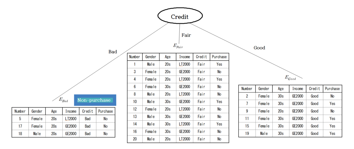
In the decision tree algorithm, the data set \(\small E\) is the data in Table 6.2.9, and the variable set is
\(\small F\) = {Gender, Age, Income, Credit}. The target variable, Purchase, has two groups, {Yes, No}.
The stopping rule of the decision tree is ‘If the number of data in each leaf is 5 or less, do not divide any more’,
and ‘If all are classified into one group, stop with the leaf as the group’.
The number of data in the current data set is 20, so stopping.conditon(\(\small E, F\)) in step 1 is false,
so go to step 6. For the root node \(\small T\)'s creatNode(), the entropy coefficient \(\small I(T) \) for
the distribution of the purchasing group(\(\small G_1\)) and the non-purchasing group (\(\small G_2\)), (8/20, 12/20), is as follows;
$$ \small
I(T) = - 0.4 \times log_{2} 0.4 - 0.6 \times log_{2} 0.6 = 0.9710
$$
In order to find the optimal branch split, find_best_split(), of step 7, a cross-table is obtained for each variable
by group, and the expected information and information gain for the variable are obtained as in Table 6.2.10
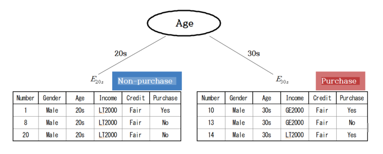
using the entropy coefficient. Since the information gain of the credit status is the largest, the root node
becomes the credit status, and the set of variable values of credit status in step 8 becomes
\(\small V\) = {Bad, Fair, Good}. The \(\small E_{Bad}, E_{Fair}, E_{Good}\) according to the credit status in step 10
are drawn in the form of a decision tree as in <Figure 6.2.3>.
| Table 6.2.10 Expected information and information gain for each variable |
| Variable |
Purchasing group \(G_1\) |
Non-purchasing group \(G_2\) |
Total |
Entropy |
Information gain
\(\Delta\) |
| Gender |
Female |
4 |
8 |
12 |
0.9183 |
| Male |
4 |
4 |
8 |
1.0000 |
| Expected entropy |
0.9510 |
0.0200 |
| Age |
20s |
2 |
8 |
10 |
0.7219 |
| 30s |
6 |
4 |
10 |
0.9710 |
| Expected entropy |
0.8464 |
0.1246 |
| Income |
GE200 |
6 |
8 |
14 |
0.9852 |
| LT200 |
2 |
4 |
6 |
0.9783 |
| Expected entropy |
0.9651 |
0.0059 |
| Credit |
Bad |
0 |
3 |
3 |
0.0000 |
| Fair |
4 |
7 |
11 |
0.9457 |
| Good |
4 |
2 |
6 |
0.9183 |
| Expected entropy |
0.9756 |
0.1754 |
<Figure 6.2.3> Decision tree with branching according to credit status
The TreeGrowth() algorithm is repeatedly applied to each data set until the stopping rule is satisfied (step 11).
Among these, the data sets of 3 people with Bad credit, \(\small E_{Bad} \), are all Non-purchasing groups, satisfying the stopping rule,
so they are not branching any further, and the leaves are marked as the Non-purchasing group.
Since the stopping rule is not satisfied for the data set of 11 people with Fair credit, \(\small E_{Fair} \),
this data set needs further split.
The entropy coefficients for the distribution (4/11, 7/11) of the Purchasing group (\(\small G_1 \)) and
the Non-purchasing group (\(\small G_2 \)) are as follows.
$$ \small
I(E_{Fair}) = - \frac{4}{11} \times log_{2} \frac{4}{11} - \frac{7}{11} \times log_{2} \frac{7}{11} = 0.9457
$$
In order to find the optimal split, find_best_split(), for the 11 people, a cross-table for each variable by the group
is obtained, and the expected information and information gain for the variables are obtained using the entropy coefficient,
as shown in Table 6.2.11. In the case of the data set with Fair credit, the information gain for Gender is the largest,
so it becomes a node for branching, and a decision tree such as <Figure 6.2.4> is formed.
| Table 6.2.11 Expected information and information gain for each variable in \(\small E_{Fair} \) |
| Variable |
Purchasing group \(G_1\) |
Non-purchasing group \(G_2\) |
Total |
Entropy |
Information gain
\(\Delta\) |
| Gender |
Female |
1 |
4 |
5 |
0.7219 |
| Male |
3 |
3 |
6 |
1.0000 |
| Expected entropy |
0.8736 |
0.0721 |
| Age |
20s |
2 |
4 |
6 |
0.9183 |
| 30s |
2 |
3 |
5 |
0.9710 |
| Expected entropy |
0.9422 |
0.0034 |
| Income |
GE200 |
2 |
4 |
6 |
0.9183 |
| LT200 |
2 |
3 |
5 |
0.9710 |
| Expected entropy |
0.9422 |
0.0034 |
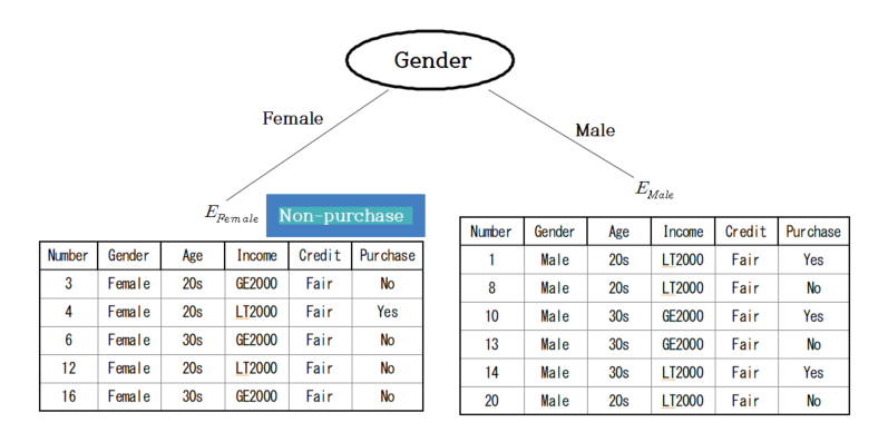
<Figure 6.2.4> Decision tree with branching according to Gender in \(\small E_{Fair} \)
As shown in the Figure 6.2.4, there are 5 data sets of Female with Fair credit, \(\small E_{Female} \), which satisfies
the stopping rule, so they are not split any further. Since there four people who did not purchase the computer and
only one person purchased, this node are marked as Non-purchasing group by majority vote.
As shown in Figure 6.2.4, there are 6 data sets of Male with Fair credit, \(\small E_{Male} \),
the stopping rule is not satisfied and this data set needs further split.
The entropy coefficients for the distribution (3/6, 3/6) of the Purchasing group (\(\small G_1 \)) and
the Non-purchasing group (\(\small G_2 \)) are as follows.
$$ \small
I(E_{Male}) = - \frac{3}{6} \times log_{2} \frac{3}{6} - \frac{3}{6} \times log_{2} \frac{3}{6} = 1
$$
In order to find the optimal branch split, find_best_split(), for the 6 people, a cross-table by the group for each variable
is obtained, and the expected information and information gain for the variables are obtained using the entropy coefficient,
as shown in Table 6.2.12. In the case of the Male with Fair credit, the information gain for Age is the largest,
so it becomes a node for branching, and a decision tree such as <Figure 6.2.5> is formed.
Here, since there are 3 people in their 20s and 30s, there is no more branching, and the 20s becomes the Non-purchasing group,
and the 30s becomes the Purchasing group by majority vote.
| Table 6.2.12 Expected information and information gain for each variable in \(\small E_{Male} \) |
| Variable |
Purchasing group \(G_1\) |
Non-purchasing group \(G_2\) |
Total |
Entropy |
Information gain
\(\Delta\) |
| Age |
20s |
1 |
2 |
3 |
0.9183 |
| 30s |
2 |
1 |
3 |
0.9183 |
| Expected entropy |
0.9183 |
0.0817 |
| Income |
GE200 |
1 |
1 |
2 |
1.0000 |
| LT200 |
2 |
2 |
4 |
1.0000 |
| Expected entropy |
1.0000 |
0.0000 |
<Figure 6.2.5> Decision tree with branching according to Gender in \(\small E_{Male} \)
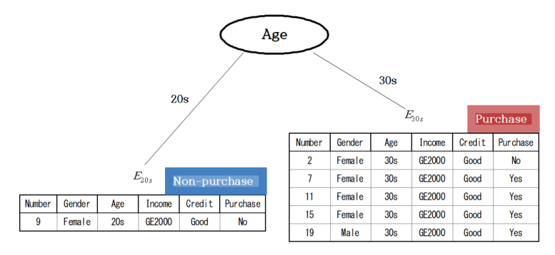
At the root node with Credit, since the stopping rule is not satisfied for the data set of 6 people with Good credit, \(\small E_{Good} \),
the entropy coefficients for the distribution (4/6, 2/6) of the Purchasing group (\(\small G_1 \)) and
the Non-purchasing group (\(\small G_2 \)) are as follows.
$$ \small
I(E_{Good}) = - \frac{4}{6} \times log_{2} \frac{4}{6} - \frac{2}{6} \times log_{2} \frac{2}{6} = 0.9183
$$
In order to find the optimal branch split, find_best_split(), for the 6 people, a cross-table by the group for each variable
is obtained, and the expected information and information gain for the variables are obtained using the entropy coefficient
as shown in Table 6.2.13. Since the information gain of Age is the largest in the data set of Good credit,
it becomes a node for branching and forms a decision tree as in <Figure 6.2.6>. As shown in the figure,
among the people with Good credit, there is only one person in Age 20s who did not purchase a computer,
so it becomes the Non-purchasing group by the stopping rule. There are 5 people in Age 30s, and 4 of them
purchased a computer, so they become the Purchasing group by majority vote.
| Table 6.2.13 Expected information and information gain for each variable in \(\small E_{Good} \) |
| Variable |
Purchasing group \(G_1\) |
Non-purchasing group \(G_2\) |
Total |
Entropy |
Information gain
\(\Delta\) |
| Gender |
Female |
3 |
2 |
5 |
0.9710 |
| Male |
1 |
0 |
1 |
0.0000 |
| Expected entropy |
0.8091 |
0.1092 |
| Age |
20s |
0 |
1 |
1 |
0.0000 |
| 30s |
4 |
1 |
5 |
0.7219 |
| Expected entropy |
0.6016 |
0.3167 |
| Income |
GE200 |
4 |
2 |
6 |
0.9183 |
| LT200 |
0 |
0 |
0 |
0.0000 |
| Expected entropy |
0.9183 |
0.0000 |
<Figure 6.2.6> Decision tree with branching according to Age in \(\small E_{Good} \)
If we combine the above, the decision tree in Figure 6.2.7 is completed. Therefore, the customer
who is a 33-year-old man, has a monthly income of 220, and has a good credit is classified as a Purchasing group.
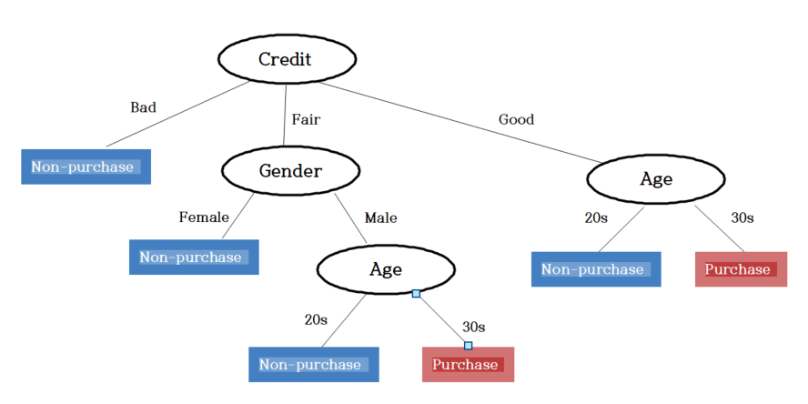
<Figure 6.2.7> Decision tree to decide a customer will purchase a computer or not
In 『eStatU』 menu, select [Decision Tree] to see the window as follows;
Check the criteria for variable selection which is 'Entropy' in this example, enter the maximum tree depth 5 and
the minimum number of data 5 for a decision. You can divide the original data set into 'Train' and 'Test'
by assigning the percents. Click [Execute] button to see the bar graph matrix and decision tree.
Click [Classification Stat] to see the decision rules of this decision tree and the accuracy/misclassification of
the classification as in <Figure 6.2.8>.
Click [Classification Table] to see the original data and classification result as in <Figure 6.2.9>.
[Decision Tree]
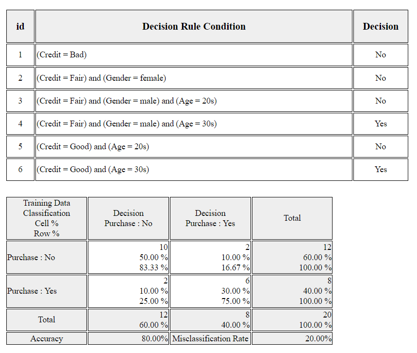
<Figure 6.2.8> Decision rules and classifcation acuracy
<Figure 6.2.9> Original data and classification
6.2.3 Categorization of a continuous variable
We can convert a continuous variable to a categorical variable, and a decision tree model can be applied.
For example, the monthly income variable can be divided into two groups: ‘Greater than or equal 2000’ and
‘Less than 2000’. In this case, the question arises ‘What boundary value should be used to divide
a value of the continuous variable?’ An expert related to this research can decide this boundary value.
However, if the determination of the boundary value is for more accurate classification, then
the uncertainty measures studied in the previous section can be used to determine the boundary value
which increases the accuracy of the classification.
Example 6.2.6
In a store, a survey of 10 customers was conducted on their monthly income (unit 10,000 won) and whether they purchased
a certain product or not, and the results are shown in Table 6.2.14. The incomes are arranged in ascending order
and the purchase status is denoted as 'Y' if a customer purchases, and 'N' if he did not purchase.
In order to apply the decision tree model, we want to divide the monthly income into two categories.
What boundary value of the income is reasonable to divide for classification?
| Table 6.2.14 Survey of customers on income and purchase status |
| Purchase | N | N | N | Y | Y | Y | N | N | N | N |
| Income | 100 | 120 | 160 | 180 | 186 | 190 | 210 | 250 | 270 | 300 |
Answer
It is reasonable to examine all middle values of two adjacent incomes as the boundary value,
and check how their classification result is made. Then select the boundary value with the least ‘uncertainty’ among them.
When a boundary value is examined, if incomes on left side of the boundary value are classified as 'N' group and incomes
on the right-side of the boundary value are classified as 'Y' group, a crosstable for classification is summarized
as in Table 6.2.15. A boundary value which is smaller than the minimum income or larger than the maximum income
is excluded because its division is meaningless. For the first middle value 110 between income 100 and 120 in Table 6.2.11,
we classify data using the rule as follows;
$$ \small
\text{If the income ≤ 110, then classify data as 'N' group, else classify data as 'Y' group}
$$
The data 100 is classified correctly using this rule as 'N' group, and the remaining nine data are classified 'Y' group,
therefore, three (180, 186, 190) out of nine data are classified correctly as 'Y' group, and six (120, 160, 210, 250, 270, 300)
out of nine data are classified incorrectly as 'Y' group as the following crosstable;
Using the Gini coefficient as the uncertainty measure, the expected Gini coefficient when the middle value
is 110 calculated as follows;
$$ \small
\frac{1}{10} \times \left\{ 1 - ( \frac{1}{1} )^2 - ( \frac{0}{1} )^2 \right\} \;+\; \frac{9}{10} \times \left\{ 1 - ( \frac{6}{9} )^2 - ( \frac{3}{9} )^2 \right\} = 0.4000
$$
The expected Gini coefficients for all remaining middle values can be calculated in the same way as Table 6.2.15.
The boundary value with the least uncertainty is 200.
| Table 6.2.15 Expected Gini coefficient using the middle value of two adjacent incomes |
|
|
Actual group |
|
| Middle value = 110 |
|
\(N\) |
\(Y\) |
Total |
Expected Gini coefficient |
| Classified group |
\(N\) |
1 |
0 |
1 |
| \(Y\) |
6 |
3 |
9 |
|
Total |
|
|
10 |
0.400 |
|
|
Actual group |
|
| Middle value = 135 |
|
\(N\) |
\(Y\) |
Total |
Expected Gini coefficient |
| Classified group |
\(N\) |
2 |
0 |
2 |
| \(Y\) |
5 |
3 |
8 |
|
Total |
|
|
10 |
0.375 |
|
|
Actual group |
|
| Middle value = 170 |
|
\(N\) |
\(Y\) |
Total |
Expected Gini coefficient |
| Classified group |
\(N\) |
3 |
0 |
3 |
| \(Y\) |
4 |
3 |
7 |
|
Total |
|
|
10 |
0.343 |
|
|
Actual group |
|
| Middle value = 183 |
|
\(N\) |
\(Y\) |
Total |
Expected Gini coefficient |
| Classified group |
\(N\) |
3 |
1 |
4 |
| \(Y\) |
4 |
2 |
6 |
|
Total |
|
|
10 |
0.417 |
|
|
Actual group |
|
| Middle value = 188 |
|
\(N\) |
\(Y\) |
Total |
Expected Gini coefficient |
| Classified group |
\(N\) |
3 |
2 |
5 |
| \(Y\) |
4 |
1 |
5 |
|
Total |
|
|
10 |
0.400 |
|
|
Actual group |
|
| Middle value = 200 |
|
\(N\) |
\(Y\) |
Total |
Expected Gini coefficient |
| Classified group |
\(N\) |
3 |
3 |
6 |
| \(Y\) |
4 |
0 |
4 |
|
Total |
|
|
10 |
0.300 |
|
|
Actual group |
|
| Middle value = 230 |
|
\(N\) |
\(Y\) |
Total |
Expected Gini coefficient |
| Classified group |
\(N\) |
4 |
3 |
7 |
| \(Y\) |
3 |
0 |
3 |
|
Total |
|
|
10 |
0.343 |
|
|
Actual group |
|
| Middle value = 260 |
|
\(N\) |
\(Y\) |
Total |
Expected Gini coefficient |
| Classified group |
\(N\) |
5 |
3 |
8 |
| \(Y\) |
2 |
0 |
2 |
|
Total |
|
|
10 |
0.375 |
|
|
Actual group |
|
| Middle value = 285 |
|
\(N\) |
\(Y\) |
Total |
Expected Gini coefficient |
| Classified group |
\(N\) |
6 |
3 |
9 |
| \(Y\) |
1 |
0 |
1 |
|
Total |
|
|
10 |
0.400 |
The method of setting the boundary value of the continuous variable, as the above example, requires many calculations.
If there are several candidates for the threshold, we can decide which of them is better in a similar way.
Example 6.2.7
In a department store, when 20 customers were surveyed, 7 (35%) made purchases and 13 (65%) did not make purchases.
A cross-tabulation was created to compare the methods of dividing the ages of these 20 people into those
under 25 and over 25, and those under 35 and over 35, as shown in Table 6.2.16. Using the entropy information gain,
decide which interval is better.
| Table 6.2.16 crosstable of two interval divisions by purchase status |
|
Purchase status |
|
| Age interval 1 |
Purchasing group |
Non-purchasing group |
Total |
| < 25 |
1 |
5 |
6 |
| \(\ge\) 25 |
6 |
8 |
14 |
| Total |
7 |
13 |
20 |
| Age interval 2 |
Purchasing group |
Non-purchasing group |
Total |
| < 35 |
3 |
12 |
15 |
| \(\ge\) 35 |
4 |
1 |
5 |
| Total |
7 |
13 |
20 |
Answer
Let us compare the two crosstables to see which interval division is better.
(Age interval 1) has many Non-purchasing groups in both '< 25' and '\(\ge 25\) intervals.
(Age unterval 2) has 12 customers in Non-purchasing group out of 15 customers who are '< 35' which is a high proportion,
and 4 customers in Purchasing group out of 5 customers who are '\(\ge 35\) which is also a high proportion.
Therefore, among the two interval division methods, (Age interval 2) provides more information on purchase.
Let us confirm this using the entropy measure.
The expected entropy for the total distribution (\( \frac{7}{20} , \frac{13}{20}\)) of Purchasing group and
Non-purchasing group is calculated as follows.
$$ \small
- (\frac{7}{20}) \; log_{2} ( \frac{7}{20} ) \; - \;(\frac{13}{20} ) \; log_{2} (\frac{13}{20} ) \;=\; 0.9341
$$
The expected entropy and information gain for the two interval divisions are calculated as in Table 6.2.17.
| Table 6.2.17 Expected entropy and information gain of two interval divisions |
|
Purchase status |
|
| Age interval 1 |
Purchasing group |
Non-purchasing group |
Total |
Entropy |
|
| < 25 |
1 |
5 |
6 |
\(\small - (\frac{1}{6}) log_{2} ( \frac{1}{6} )^2 - (\frac{5}{6} ) log_{2} (\frac{5}{6} ) = 0.6500\) |
| \(\ge\) 25 |
6 |
8 |
14 |
\(\small - (\frac{6}{14}) log_{2} ( \frac{6}{14} )^2 - (\frac{8}{14} ) log_{2} (\frac{8}{14} ) = 0.9852\) |
| Total |
7 |
13 |
20 |
Expected entropy
= \(\small \frac{6}{20} \times 0.6500 + \frac{14}{20} \times 0.9852\)
= 0.8847 |
Information gain
= \(\small 0.9341 - 0.8847\)
= 0.0494 |
| Age interval 2 |
Purchasing group |
Non-purchasing group |
Total |
Entropy |
|
| < 35 |
3 |
12 |
15 |
\(\small - (\frac{3}{15}) log_{2} ( \frac{3}{15} )^2 - (\frac{12}{15} ) log_{2} (\frac{12}{15} ) = 0.7219\) |
| \(\ge\) 35 |
4 |
1 |
5 |
\(\small - (\frac{4}{5}) log_{2} ( \frac{4}{5} )^2 - (\frac{1}{5} ) log_{2} (\frac{1}{5} ) = 0.7219\) |
| Total |
7 |
13 |
20 |
Expected entropy
= \(\small \frac{15}{20} \times 0.7219 + \frac{5}{20} \times 0.7219\)
= 0.7219 |
Information gain
= \(\small 0.9341 - 0.7219\)
= 0.2121 |
(Age interval 2) that divides into '< 35' and '\(\ge\) 35' has a large information gain, so this interval division
is selected.
The above method can also be applied if you want to reduce the number of categories when there are multiple values
for a categorical variable. For example, if there are three categorical variable values, (\(A_{1}, A_{2}, A_{3}\)),
and we want to reduce them to two, we can investigate the information gain for the three possible combinations
(\(A_{1}, A_{2} : A_{3}\)), (\(A_{1}, A_{3} : A_{2}\)), (\(A_{2}, A_{3} : A_{1}\)) and select the combination
that maximizes the information gain.
6.2.4 Overfitting and pruning decision tree
Decision tree models can have an overfitting problem, classifying training data well but not good for testing data.
Pruning is one way to solve the problem of overfitting, and there are pre-pruning and post-pruning. Pre-pruning
is to examine the appropriateness of the division using chi-square tests and information gain to prevent
meaningless divisions from continuing. Regardless of which method is applied, a threshold value must be set,
which must be determined by the researcher. If the threshold value is too high, a simple tree will be formed,
and conversely, if it is too low, a complex tree may be formed.
Post-pruning is a method of removing branches from a completed tree. For example, when pruning subtrees
for each node, the expected error rate is calculated, and if this value is the maximum expected error rate,
the subtrees are maintained. Otherwise, they are pruned. Pre-pruning and post-pruning are sometimes used in combination.
Characteristics of decision tree model
The important characteristics of the decision tree classification model are summarized as follows:
1) The decision tree model is a nonparametric method that does not assume the distribution function of each group.
2) The results of the decision tree model are easy to explain to anyone. The accuracy of the model is not inferior to other classification models.
3) Since the method of creating a decision tree is not computationally complex, it can be created quickly, even for large amounts of data. Once a decision tree is created, the task of classifying data whose group affiliation is unknown into one group is very fast.
4) The decision tree algorithm can classify abnormal noise data without much sensitivity.
5) Even if there are other unnecessary variables that are highly correlated with one variable, the decision tree
is not greatly affected. However, if there are many unnecessary variables, there is a risk that the decision tree
will become too large. It is necessary to remove unnecessary variables before classification to prevent the risk.
6) Since the number of decision trees that can be created from one data is very large, it is not easy to find
the optimal decision tree among them. Most decision tree algorithms use heuristic search to find the optimal tree,
and the Algorithm we discussed also expands the decision tree using a top-down iterative partitioning strategy.
7) Since most decision tree algorithms are top-down iterative partitioning algorithms, they continuously partition
the entire data set into smaller data sets. If this process is repeated, there may be too few data in some leaves
to make a statistically meaningful classification decision. It is necessary to create a stopping rule that
prevents further partitioning when the number of data in a node is less than a certain number.
8) In the entire decision tree, small trees (subtrees) with the same shape can appear in multiple nodes,
which can complicate the decision tree.
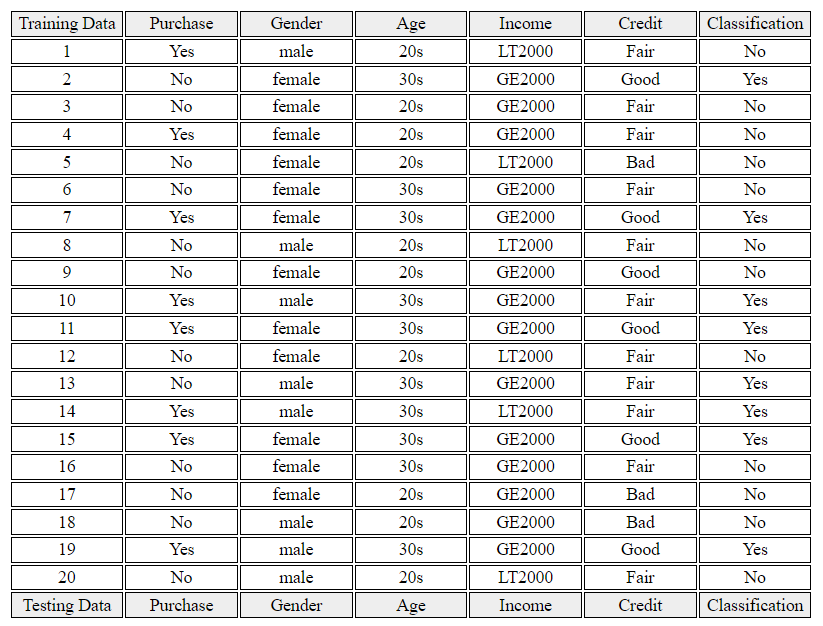
9) A decision tree examines only the conditions for one variable in one node. Therefore, the classification rule
of the decision tree partitions the entire decision space into straight lines parallel to the coordinate axes (variables)
(<Figure 6.2.10>).
<Figure 6.2.10> Split two dimension decision space by a decision tree
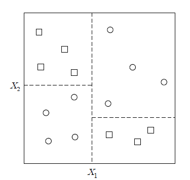
However, the example data in <Figure 6.2.11> is not easy to split by a decision tree.
The test condition at the node can be transformed into one for more than one variable to solve the problem,.
For example, a diagonal shape like <Figure 6.2.11> can be considered as a test condition for two variables.
It would be good to create a test condition for more than two variables, but the calculation is complicated
and another problem of ‘how to create the optimal test condition?’ arises.
<Figure 6.2.11> Example data which is not easy to split by a decision tree
10) The choice of uncertainty measures such as entropy or Gini coefficient does not have a significant effect
on the performance of the decision tree. This is because the measures have similar characteristics.
What affects the performance of the decision tree is the choice of the tree pruning method rather than
the choice of measure.
6.2.5 R and Python practice
Let us practice R commands using the data saved at http://estat.me/estat/Example/DataScience/PurchaseByCredit20.csv.
The file format is a comma separated value (csv) type. You can find this file
from 『eStat』 system. Click Ex > DataScience and then click the data 'PurchaseByCredit20.csv'.
After this file is loaded to 『eStat』, save it using 'csv Save' button. It will be
saved at the Download folder on your PC. Copy this file to C:\Rwork\ folder.
In order to practice the decision tree using this data, you need to change first the working directory of R
as follows.
File > Change Directory > C: > Rwork
If you read the data file in R, it looks like as follows.
| # read the data file |
| card <- read.csv("http://estat.me/estat/Example/DataScience/PurchaseByCredit20.csv", header=T, as.is=FALSE) |
card
      id Gender Age Income Credit Purchase
1      1   male 20s LT2000   Fair      Yes
2      2 female 30s GE2000   Good       No
3      3 female 20s GE2000   Fair       No
4      4 female 20s GE2000   Fair      Yes
5      5 female 20s LT2000    Bad       No
6      6 female 30s GE2000   Fair       No
7      7 female 30s GE2000   Good      Yes
8      8   male 20s LT2000   Fair       No
9      9 female 20s GE2000   Good       No
10    10   male 30s GE2000   Fair      Yes
11    11 female 30s GE2000   Good      Yes
12    12 female 20s LT2000   Fair       No
13    13   male 30s GE2000   Fair       No
14    14   male 30s LT2000   Fair      Yes
15    15 female 30s GE2000   Good      Yes
16    16 female 30s GE2000   Fair       No
17    17 female 20s GE2000    Bad       No
18    18   male 20s GE2000    Bad       No
19    19   male 30s GE2000   Good      Yes
20    20   male 20s LT2000   Fair       No
|
| attach(card) |
To analyze decision trees using R, you need to install a package called
rpart. From the main menu of R,
select ‘Package’ => ‘Install package(s)’, and a window called ‘CRAN mirror’ will appear. Here,
select ‘0-Cloud [https]’ and click ‘OK’. Then, when the window called ‘Packages’ appears, select
‘rpart’ and click ‘OK’.
'rpart' is a package for modeling of Recursive Partitioning and Regression Trees and general usage and
key arguments of the function are described in the following table.
Fit a Recursive Partitioning and Regression Trees
|
|
rpart(formula, data, weights, subset, na.action = na.rpart, method, model = FALSE, x = FALSE, y = TRUE, parms, control, cost, ...)
|
| formula |
a formula, with a response but no interaction terms. If this a a data frame, that is taken as the model frame (see model.frame). |
| data |
an optional data frame in which to interpret the variables named in the formula. |
| method |
one of "anova", "poisson", "class" or "exp". If method is missing then the routine tries to make an intelligent guess. If y is a survival object, then method = "exp" is assumed, if y has 2 columns then method = "poisson" is assumed, if y is a factor then method = "class" is assumed, otherwise method = "anova" is assumed. It is wisest to specify the method directly, especially as more criteria may added to the function in future. |
| parms |
optional parameters for the splitting function.
Anova splitting has no parameters.
Poisson splitting has a single parameter, the coefficient of variation of the prior distribution on the rates. The default value is 1.
Exponential splitting has the same parameter as Poisson.
For classification splitting, the list can contain any of: the vector of prior probabilities (component prior), the loss matrix (component loss) or the splitting index (component split). The priors must be positive and sum to 1. The loss matrix must have zeros on the diagonal and positive off-diagonal elements. The splitting index can be gini or information. The default priors are proportional to the data counts, the losses default to 1, and the split defaults to gini.
|
| control |
a list of options that control details of the rpart algorithm. See rpart.control. |
| rpart.control(minsplit = 20, minbucket = round(minsplit/3), cp = 0.01,
maxcompete = 4, maxsurrogate = 5, usesurrogate = 2, xval = 10,
surrogatestyle = 0, maxdepth = 30, ...)
|
| minsplit |
the minimum number of observations that must exist in a node in order for a split to be attempted. |
| minbucket |
the minimum number of observations in any terminal node. If only one of minbucket or minsplit is specified, the code either sets minsplit to minbucket*3 or minbucket to minsplit/3, as appropriate. |
| cp |
complexity parameter. Any split that does not decrease the overall lack of fit by a factor of cp is not attempted. For instance, with anova splitting, this means that the overall R-squared must increase by cp at each step. The main role of this parameter is to save computing time by pruning off splits that are obviously not worthwhile. Essentially,the user informs the program that any split which does not improve the fit by cp will likely be pruned off by cross-validation, and that hence the program need not pursue it. |
| maxdepth |
Set the maximum depth of any node of the final tree, with the root node counted as depth 0. Values greater than 30 rpart will give nonsense results on 32-bit machines.
|
An example of R commands for a decision tree using the dataset card is as follows.
The results of practicing a decision tree in R with purchase as the dependent variable of card data
and other variables as independent variables are as follows. In Example 6.2.5, the information gain
of credit status was the largest, so this variable was the root node. However, since some of the number of data
belonging to credit status variable value was small (‘bad’ = 3, ‘good’ = 6, ), the next largest information gain,
which is age, was selected as the root node in R.
| install.packages('rpart') |
| library(rpart) |
| fit <- rpart(Purchase ~ Gender + Age + Income + Credit, data = card) |
fit
n= 20
node), split, n, loss, yval, (yprob)
      * denotes terminal node
1) root 20 8 No (0.6000000 0.4000000)
  2) Age=20s 10 2 No (0.8000000 0.2000000) *
  3) Age=30s 10 4 Yes (0.4000000 0.6000000)
|
However, the analysis result is simple because the minimum number of pruning data of the rpart function is 20
or more by default. Let's change this default setting and prune it.
The results of practicing decision trees in R with purchase as the dependent variable of card data
and other variables as independent variables are as follows.
| fit2 <- rpart(Purchase ~ Gender + Age + Income + Credit, data = card, control = rpart.control(minsplit = 6)) |
fit2
n= 20
node), split, n, loss, yval, (yprob)
      * denotes terminal node
1) root 20 8 No (0.6000000 0.4000000)
  2) Age=20s 10 2 No (0.8000000 0.2000000) *
  3) Age=30s 10 4 Yes (0.4000000 0.6000000)
    6) Credit=Fair 5 2 No (0.6000000 0.4000000) *
    7) Credit=Good 5 1 Yes (0.2000000 0.8000000) *
|
To draw a decision tree as a graph, use the plot and text commands below.
'plot' draws a tree diagram and, if the option 'compress' is T, the vertical width is narrowed,
and if 'uniform' is T, the horizontal width is narrowed. 'margin' sets the margin.
If the margin is 0, the label may be cut off, so set it little by little.
'text' labels the tree, and 'use.n' displays something like 0/4. The decision tree drawn with the above command is as follows.
| plot(fit2,compress=T,uniform=T,margin=0.1) |
text(fit2,use.n=T,col='blue')
<Figure 6.2.12> Decision tree using R
|
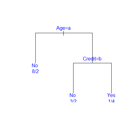
In the decision tree diagram above, age=a is the condition of the left branch, and 'a' means the first variable value '20s',
credit=b is also the condition of the left branch, and 'b' means 'fair'
(in this case, it seems to have been merged because 'bad' is missing).
For more information, please refer to the help. In packages such as R, when the number of data corresponding to each variable value
is too small, pruning is determined by merging with adjacent variable values.
Python practice
[Colab]
# Import required libraries
import pandas as pd
import matplotlib.pyplot as plt
# Read the data file
url = 'https://raw.githubusercontent.com/ogut77/DataScience/refs/heads/main/PurchaseByCredit40.csv'
card = pd.read_csv(url)
# Display the data
print(card)
    id  Gender  Age  Income Credit Purchase
0    1    male  20s  LT2000   Fair      Yes
1    2  female  30s  GE2000   Good       No
2    3  female  20s  GE2000   Fair       No
3    4  female  20s  GE2000   Fair      Yes
4    5  female  20s  LT2000    Bad       No
5    6  female  30s  GE2000   Fair       No
6    7  female  30s  GE2000   Good      Yes
7    8    male  20s  LT2000   Fair       No
8    9  female  20s  GE2000   Good       No
9   10    male  30s  GE2000   Fair      Yes
10  11  female  30s  GE2000   Good      Yes
11  12  female  20s  LT2000   Fair       No
12  13    male  30s  GE2000   Fair       No
13  14    male  30s  LT2000   Fair      Yes
14  15  female  30s  GE2000   Good      Yes
15  16  female  30s  GE2000   Fair       No
16  17  female  20s  GE2000    Bad       No
17  18    male  20s  GE2000    Bad       No
18  19    male  30s  GE2000   Good      Yes
19  20    male  20s  LT2000   Fair       No
20  21    male  20s  LT2000   Fair      Yes
21  22  female  30s  GE2000   Good       No
22  23  female  20s  GE2000   Fair       No
23  24  female  20s  GE2000   Fair      Yes
24  25  female  20s  LT2000    Bad       No
25  26  female  30s  GE2000   Fair       No
26  27  female  30s  GE2000   Good      Yes
27  28    male  20s  LT2000   Fair       No
28  29  female  20s  GE2000   Good       No
29  30    male  30s  GE2000   Fair      Yes
30  31  female  30s  GE2000   Good      Yes
31  32  female  20s  LT2000   Fair       No
32  33    male  30s  GE2000   Fair       No
33  34    male  30s  LT2000   Fair      Yes
34  35  female  30s  GE2000   Good      Yes
35  36  female  30s  GE2000   Fair       No
36  37  female  20s  GE2000    Bad       No
37  38    male  20s  GE2000    Bad       No
38  39    male  30s  GE2000   Good      Yes
39  40    male  20s  LT2000   Fair       No
# Prepare the data
y=card['Purchase']
X=card.drop(['Purchase'], axis=1)
# X=pd.get_dummies(X,drop_first=True)
# Prepare the data
for column in X.select_dtypes(include=['object']).columns:
X[column] = label_encoder.fit_transform(X[column])
# Create and train the decision tree model
dt = DecisionTreeClassifier()
fit = dt.fit(X, y)
fit
DecisionTreeClassifier()
In a Jupyter environment, please rerun this cell to show the HTML representation or trust the notebook.
On GitHub, the HTML representation is unable to render, please try loading this page with nbviewer.org.
dt = DecisionTreeClassifier(min_samples_split=6, random_state=42) #Added random_state for reproducibility
fit2 = dt.fit(X, y) #Fit on the training data
fit2
DecisionTreeClassifier(min_samples_split=6, random_state=42)
In a Jupyter environment, please rerun this cell to show the HTML representation or trust the notebook.
On GitHub, the HTML representation is unable to render, please try loading this page with nbviewer.org.
# prompt: plot(fit2,compress=T,uniform=T,margin=0.1)
# text(fit2,use.n=T,col='blue') in python
import matplotlib.pyplot as plt
from sklearn.tree import plot_tree
# Assuming 'fit2' is your trained DecisionTreeClassifier object and X, y are defined as in your previous code
plt.figure(figsize=(20,10)) # Adjust figure size as needed
plot_tree(fit2, filled=True, feature_names=X.columns, class_names=True, rounded=True) #filled=True is similar to compress=T, rounded=True is similar to uniform=T
plt.show()
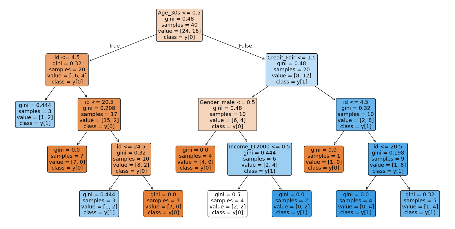
|
6.3 Naive Bayes classification model
6.3.1 Bayes classification
When the prior probability of being classified into each group and the likelihood probability
of each group are known, the Bayes classification model is a method of classifying data into groups
with high probability by calculating the posterior probability using Bayes theorem, which was introduced
in section 4.1.2. Let us look at the Bayes classification model for a single variable case using the following example.
Example 6.3.1 (Classification by prior probability)
When 20 customers who visited a computer store were surveyed, 8 customers purchased a computer, and 12 customers
did not purchase a computer. Based on this information, classify a customer who visited this store on a day
whether he would purchase a computer or not.
Answer
Among the 20 customers who visited the store, only 8 (40%) purchased a computer, and 12 (60%) did not purchase a computer.
This information, the probability of the purchasing group is 40% and the probability of the non-purchasing
group is 60% by surveying past data, are called prior probabilities. If a decision is made based on
these prior probabilities, since the probability of the non-purchasing group is higher than the purchasing group,
it is reasonable to classify a customer who visited on a day as into the non-purchasing group.
As in the example above, classifying data whose group membership is unknown
into a group with the highest prior probability is called a classification by prior probability.
If the purchasing group of the computer is \(G_{1}\) and the non-purchasing group is \(G_{2}\), and the
prior probability of each group is \(P(G_{1})\) and \(P(G_{2})\), the classification rule by the prior probability is as follows;
Classification rule by prior probability
\(\qquad\)‘If \(P(G_{1})\) ≥ \(P(G_{2})\), classify the data into group \(G_{1}\), otherwise classify it into \(G_{2}\)’
If we can obtain the distribution of the age of the purchasing group and the non-purchasing group, it can be
useful information for judging whether to purchase or not. This is called the likelihood probability distribution
or group probability distribution. In this case, we can calculate the posterior probability of each group
using the Bayes theorem, and the classification using this posterior probability is called Bayes classification.
Let us look at the following example.
Example 6.3.2 (Classification by posterior probability)
In Example 6.3.1, the classification decision was made using simple prior information such as the probability of
the purchasing group and the non-purchasing group. One of the additional information that can be obtained is
a customer's age. Suppose there are 10 customers in their age 20's
among 20 customers and 10 customers in their age 30's. Among the 8 purchasing groups, 2 customers in their age 20's
and 6 are in their age 30's. If a customer who visited the store on a day is in his age 20's, classify the customer
whether he purchases the computer or not by calculating the posterior probability.
Answer
The customer's age by the purchasing group (\(\small G_{1}\)) and the non-purchasing group (\(\small G_{2}\))
are summarized in the following table.
| Table 6.3.1 crosstable on Age by Purchasing status |
| Age |
Purchasing group
\(\small G_{1}\) |
Non-purchasing group
\(\small G_{2}\) |
Total |
| 20's |
2 |
8 |
10 |
| 30's |
6 |
4 |
10 |
| Total |
8 |
12 |
20 |
Looking at this table, we can see that the purchasing group (\(\small G_{1}\)) has a higher proportion of customers
in age 30's, and the non-purchasing group (\(\small G_{2}\)) has a higher proportion of customers in their age 20's.
The age distribution of each group is called the likelihood probability distribution.
When the age of 20's is represented as \(\small X\), the probability of age 20s in the purchasing group is 2/8,
which is denoted as the conditional probability \(\small P( X | G_{1} ) \) and the probability of age 20's
in the non-purchasing group is 8/12, which is denoted as \(\small P( X | G_{2} ) \).
If a customer who visited on a day was in his age 20's, the probability that this customer would purchase the computer
is called the posterior probability of the purchasing group and is denoted as \(\small P( G_{1} | X ) \).
This posterior probability can be obtained as follows using Bayes' theorem.
$$ \small
\begin{align}
P( G_{1} | X ) &= \frac {P( G_{1} ) \times P(X|G_{1}) }{P( G_{1} ) \times P(X|G_{1}) + P( G_{2} ) \times P(X|G_{2})} \\
&= \frac{ \frac{8}{20} \times \frac{2}{8} }{ \frac{8}{20} \times \frac{2}{8} + \frac{12}{20} \times \frac{8}{12} } = 0.2
\end{align}
$$
Here, the denominator is the probability of all age 20's, \(\small P( X ) \) = 10/20, and the numerator means
the proportion of age 20's who purchased the computer, 2/20. In the same way, the posterior probability of
non-purchasing goup among age 20's is denoted as \(\small P( G_{2} | X ) \), and is calculated as follows using Bayes' theorem.
$$ \small
\begin{align}
P( G_{2} | X ) &= \frac {P( G_{2} ) \times P(X|G_{2}) }{P( G_{1} ) \times P(X|G_{1}) + P( G_{2} ) \times P(X|G_{2})} \\
&= \frac{ \frac{12}{20} \times \frac{8}{12} }{ \frac{8}{20} \times \frac{2}{8} + \frac{12}{20} \times \frac{8}{12} } = 0.8
\end{align}
$$
Therefore, since the posterior probability that a customer in age 20's belongs to the non-purchasing group is 0.8,
which is higher than the posterior probability of belonging to the purchasing group of 0.2, this customer is
classified as a non-purchasing group. As a result, when we obtain additional information that the visitor is in age 20's,
we can see that the probability that this person belongs to the purchasing group of 0.2 is lower than the
prior probability of 0.4.
When we know that a customer who visited is age 20's (\(\small X\)), we calculate the posterior probability
\(\small P( G_{1} | X ) \) that he belongs to the purchasing group (\(\small G_{1}\)) and the posterior probability
\(\small P( G_{2} | X ) \) that he belongs to the non-purchasing group (\(\small G_{2}\)) and classify the person
into the group with the higher posterior probability. This is called Bayes classification and the rule
can be summarized as follows.
Bayes classification rule by posterior probability
\(\qquad\) ‘If \(\small P( G_{1} | X ) \) ≥ \(\small P( G_{2} | X ) \), classify data as \(\small G_{1}\), otherwise classify as \(\small G_{2}\)’
Here, \(\small P( G_{1} | X ) \) and \(\small P( G_{2} | X ) \) have the same denominator in the calculation
of the posterior probability, so the classification rule can be written as follows.
\(\qquad\) ‘If \(\small \frac{P( X | G_{1} )}{P( X | G_{2} )} \) ≥ \(\small \frac{P(G_{2})}{P(G_{1})} \), classify data as \(\small G_{1}\), otherwise classify as \(\small G_{2}\)’
The Bayes classification model for one variable can be easily extended to the case of \(m\) random variables
\(\small \boldsymbol X = (X_{1}, X_{2}, ... , X_{m}) \). Let the prior probabilities of \(k\) number of groups,
\(\small G_{1}, G_{2}, ... , G_{k}\), be \(\small P(G_{1}), P(G_{2}), ... , P(G_{k})\), and let the likelihood
probability distribution function for each group be
\(\small P( \boldsymbol X | G_{1}), P( \boldsymbol X | G_{2}), ... , P( \boldsymbol X | G_{k})\).
Given the observation data \(\small \boldsymbol x\) for classification, the posterior probability
\(\small P(G_{i} | \boldsymbol x)\) that this data comes from the group \(\small G_{i}\) is as follows.
$$ \small
P( G_{i} | \boldsymbol x ) = \frac {P( G_{i} ) \times P(\boldsymbol x | G_{i})}{P(G_{1}) \times P(\boldsymbol x |G_{1}) + P(G_{2}) \times P(\boldsymbol x | G_{2}) + \cdots + P(G_{k}) \times P(\boldsymbol x | G_{k}) }
$$
The Bayes classification rule using the posterior probability is as follows.
Bayes Classification - multiple groups
Suppose that prior probabilities of \(k\) number of groups, \(\small G_{1}, G_{2}, ... , G_{k}\), are
\(\small P(G_{1}), P(G_{2}), ... , P(G_{k})\), and likelihood probability distribution functions
for each group are \(\small P( \boldsymbol X | G_{1}), P( \boldsymbol X | G_{2}), ... , P( \boldsymbol X | G_{k})\).
Given the observation data \(\small \boldsymbol x\) for classification, let the posterior probabilities
that \(\small \boldsymbol x\) comes from each group be
\(\small P(G_{1} | \boldsymbol x), P(G_{2} | \boldsymbol x), ... , P(G_{k} | \boldsymbol x)\).
The Bayes classification rule is as follows.
\(\qquad\) 'Classify \(\boldsymbol x\) into a group with the highest posterior probability'
If we denote the likelihood probability functions as
\(\small f_{1}(\boldsymbol x), f_{2}(\boldsymbol x), ... , f_{k}(\boldsymbol x)\),
since the denominators in the calculation of posterior probabilities are the same, the Bayes classification rule
can be written as follows.
\(\qquad\) 'If \(\small P(G_{k}) f_{k}(\boldsymbol x) ≥ P(G_{i}) f_{i}(\boldsymbol x) \) for all \(k\) ≠ \(i\),
classify \(\boldsymbol x\) into group \(\small G_{k}\)'
If there are only two groups \(\small G_{1}\)and \(\small G_{2}\), the Bayes classification rule is expressed as follows.
\(\qquad\) 'if \( \frac{f_{1}(\boldsymbol x)}{f_{2}(\boldsymbol x)} ≥ \frac{P(G_{2})}{P(G_{1})} \),
classify \(\boldsymbol x\) into group \(\small G_{1}\), else into group \(\small G_{2}\)'
When there are sample data, if the likelihood probability distribution \(f_{1}(\boldsymbol x)\) can be estimated
from the sample, the Bayes classification rule can also be estimated using the likelihood probability distribution.
Therefore, the Bayes classification rule can appear in many variations depending on the estimation method of
the likelihood probability distribution. Estimation of the likelihood probability distribution using samples
can be done using either a parametric method, such as maximum likelihood estimation, or a nonparametric method.
In the case of categorical data, a multidimensional distribution estimated from the sample is often used,
and in the case of continuous data, a multivariate normal distribution is often used.
For more information, please refer to the related references.
6.3.2 Naive Bayes classification model for categorical data
When there are two or more categorical variables for classification, if the variables can be assumed independent,
the Bayes classification is called a naive Bayes classification. In the case of categorical data,
since there are many cases in which variables can be assumed independent in real applications,
the naive Bayes classification is used frequently. Let us consider an example of the naive Bayes classification.
Example 6.3.3
Consider a survey of 20 customers at a computer store on age (\(\small X_{1}\)), monthly income (\(\small X_{2}\)),
credit status (\(\small X_{3}\)) and their purchasing status as shown in Table 6.3.2.
Note that the age transformed into '20s' and '30s' as categorical, income into 'LT2000' and 'GE2000',
and credit status into 'Bad', 'Fair' and 'Good'.
| Table 6.3.2 Survey of customers on age, income, credit status and purchasing status |
| Number |
Age |
Income
(unit USD) |
Credit |
Purchase |
| 1 | 20s | LT2000 | Fair | Yes |
| 2 | 30s | GE2000 | Good | No |
| 3 | 20s | GE2000 | Fair | No |
| 4 | 20s | GE2000 | Fair | Yes |
| 5 | 20s | LT2000 | Bad | No |
| 6 | 30s | GE2000 | Fair | No |
| 7 | 30s | GE2000 | Good | Yes |
| 8 | 20s | LT2000 | Fair | No |
| 9 | 20s | GE2000 | Good | No |
| 10 | 30s | GE2000 | Fair | Yes |
| 11 | 30s | GE2000 | Good | Yes |
| 12 | 20s | LT2000 | Fair | No |
| 13 | 30s | GE2000 | Fair | No |
| 14 | 30s | LT2000 | Fair | Yes |
| 15 | 30s | GE2000 | Good | Yes |
| 16 | 30s | GE2000 | Fair | No |
| 17 | 20s | GE2000 | Bad | No |
| 18 | 20s | GE2000 | Bad | No |
| 19 | 30s | GE2000 | Good | Yes |
| 20 | 20s | LT2000 | Fair | No |
If a customer who visited this store one day is 33 years old, has a monthly income of 1900 USD, and has a good credit status,
classify him using the posterior probability of whether he will buy a computer or not.
Answer
The one-dimensional likelihood probability distributions,
\(\small P(X_{1} | G_{i}),\; P(X_{2} | G_{i}),\; P(X_{3} | G_{i})\), of each variable by purchasing group
(\(\small G_{1}\)) and non-purchasing group (\(\small G_{1}\)) are summarized as in Table 6.3.3,
and the multidimensional likelihood probability distribution of three variables,
\(\small P((X_{1}, X_{2}, X_{3}) | G_{i})\), is summarized as in Table 6.3.4.
| Table 6.3.3 One-dimensional likelihood probability distributions on Age, Income and Credit |
| Age |
Purchasing group
\(\small G_{1}\) |
Non-purchasing group
\(\small G_{2}\) |
Total |
| 20's |
2 |
8 |
10 |
| 30's |
6 |
4 |
10 |
| Total |
8 |
12 |
20 |
| |
| Income |
Purchasing group
\(\small G_{1}\) |
Non-purchasing group
\(\small G_{2}\) |
Total |
| LT2000 |
2 |
4 |
6 |
| GE2000 |
6 |
8 |
14 |
| Total |
8 |
12 |
20 |
| |
| Credit |
Purchasing group
\(\small G_{1}\) |
Non-purchasing group
\(\small G_{2}\) |
Total |
| Bad |
0 |
3 |
3 |
| Fair |
4 |
7 |
11 |
| Good |
4 |
2 |
6 |
| Total |
8 |
12 |
20 |
| Table 6.3.4 Multi-dimensional likelihood probability distributions on Age, Income and Credit |
| Age |
Income |
Credit |
Purchasing group
\(\small G_{1}\) |
Non-purchasing group
\(\small G_{2}\) |
Total |
| 20's |
LT2000 |
Bad |
|
1 |
1 |
| Fair |
1 |
3 |
4 |
| Good |
|
|
|
| GE2000 |
Bad |
|
2 |
2 |
| Fair |
1 |
1 |
2 |
| Good |
|
1 |
1 |
| 30's |
LT2000 |
Bad |
|
|
|
| Fair |
1 |
|
1 |
| Good |
|
|
|
| GE2000 |
Bad |
|
|
|
| Fair |
1 |
3 |
4 |
| Good |
4 |
1 |
5 |
| Total |
|
|
8 |
12 |
20 |
If a customer who visited the computer store is represented as \( \boldsymbol x\) =
(\(\small x_{1}, x_{2}, x_{3}\)) = (30s, LT2000, Fair), the posterior probability
that this customer belongs to the purchasing group \(\small G_{1}\) is \(\small P(G_{1} | \boldsymbol x )\)
and the posterior probability that this customer belongs to the non-purchasing group \(\small G_{2}\) is
\(\small P(G_{2} | \boldsymbol x )\). However, in the multidimensional likelihood distribution for
the three variables in Table 6.3.4, the probability of a customer being in their 30s, with an income of LT2000,
and with fair credit is \(\small P(G_{1} | \boldsymbol x )\) = 1/8 and \(\small P(G_{2} | \boldsymbol x )\) = 0.
If the number of samples is insufficient, it is difficult to correctly estimate the likelihood probability distribution.
In this case, if variables, age, income, and credit status, can be assumed to be independent,
the one-dimensional likelihood probability distribution of each variable is used approximately to estimate
the multidimensional likelihood probability distribution as follows.
\( \qquad \small
P(\boldsymbol X = (X_{1}, X_{2}, X_{3})\; |\; G_{i}) ≈ P(X_{1} | G_{i}) \; P(X_{2} | G_{i}) \; P(X_{3} | G_{i})
\)
For this problem, the approximate likelihood of customer \(\boldsymbol x\) = (30s, LT2000, Fair) is as follows.
\( \qquad \small
P(\boldsymbol x = (30s, LT2000, Fair) \;|\; G_{1}) ≈ \frac{6}{8} \times \frac{2}{8} \times \frac{4}{8} = 0.0938
\)
\( \qquad \small
P(\boldsymbol x = (30s, LT2000, Fair) \;|\; G_{2}) ≈ \frac{4}{12} \times \frac{4}{12} \times \frac{7}{12} = 0.0648
\)
Therefore, the posterior probability for each group is as follows.
\( \qquad \small
\begin{align}
P( G_{1} | \boldsymbol x ) &= \frac {P( G_{1} ) \times P(\boldsymbol x | G_{1}) }{P( G_{1} ) \times P(\boldsymbol x | G_{1}) + P( G_{2} ) \times P(\boldsymbol x | G_{2})} \\
&= \frac{ 0.4 \times 0.0938 }{ 0.4 \times 0.0938 + 0.6 \times 0.0648 } = 0.4911
\end{align}
\)
\( \qquad \small
\begin{align}
P( G_{2} | \boldsymbol x ) &= \frac {P( G_{2} ) \times P(\boldsymbol x | G_{2}) }{P( G_{1} ) \times P(\boldsymbol x | G_{1}) + P( G_{2} ) \times P(\boldsymbol x | G_{2})} \\
&= \frac{ 0.6 \times 0.0648 }{ 0.4 \times 0.0938 + 0.6 \times 0.0648 } = 0.5089
\end{align}
\)
Since the posterior probability of belonging to the non-purchasing group is 0.5089, which is greater than
the probability of belonging to the purchasing group, which is 0.4911, the customer is classified as
the non-purchasing group. Lift chart, confusion matrix and ROC graph are to evaluate the classification
model, and they will be explained in the next section.
[]
As in the example above, assuming that variables for classification are independent,
obtaining an approximate likelihood probability distribution by group, obtaining the posterior probability,
and then classifying is called a
naive Bayes classification. The naive Bayes classification
is less realistic because it assumes that all variables are independent of each other, but it is often used
as an approximate classification method. However, you should know that it can show inaccurate classification results
when variables are related to each other.
To compensate for the problem of assuming that all variables are independent,
subsets of variables can be assumed to be independent, and the likelihood probability
distribution can be obtained. This classification model is called a Bayes belief network.
In this method, it is necessary to first investigate which variables are related to each other and
which variables are independent. For more information, please refer to the references.
6.3.3 Stepwise variable selection
Bayes classification can be applied to whether the variables are continuous or discrete, and an appropriate likelihood
probability distribution can be estimated. If continuous and discrete variables are mixed, the naive Bayes classification
can be applied by categorizing the continuous variables, as we discussed in section 6.2.3.
If there are many variables in the data, in general, we use variables that can best explain group variables,
that is, variables with high discriminatory power between groups.
A stepwise variable selection can be helpful in classifying data to increase accuracy.
There are two methods to select variables: forward selection and
backward elimination. The forward selection of variables is similar to the variable selection in
a decision tree, which selects a variable with the highest information gain using the uncertainty measures
or chi-square test. After selecting a variable for classification, add another variable with the next highest
information gain in the selection step-by-step until finding a set of variables with the highest classification accuracy.
The backward elimination initially includes all variables for classification and selects a variable to remove
from the set of all variables, which can improve classification accuracy. Continue removing a variable
from the set of variables until there is no improvement in classification accuracy. The chi-square test,
which we discussed in section 6.2.2 is often used for this backward selection of variables in naive Bayes classification.
A stepwise method also selects variables using the forward selection method while examining
whether the variables already selected can be removed. However, it is not easy to verify whether the ‘optimal’
variable selection was made regardless of the method used. For more information, please refer to the references.
Characteristics of Bayes classification model
The characteristics of Bayes classification are summarized as follows.
1) Since the Bayes classification model classifies using the posterior probability, which is calculated by
the prior probability and the likelihood probability distribution of each group, the risk of overfitting
the model is low but robust.
2) Bayes classification model can perform stable classification even when there are incomplete data,
outliers, and missing values.
6.3.4 R and Python practice - Naive Bayes classification
To analyze naive Bayes classification using R, you need to install a package called
naivebayes.
From the main menu of R,
select ‘Package’ => ‘Install package(s)’, and a window called ‘CRAN mirror’ will appear. Here,
select ‘0-Cloud [https]’ and click ‘OK’. Then, when the window called ‘Packages’ appears, select
‘naivebayes’ and click ‘OK’.
'naivebayes' is a package for modeling of Naive Bayes model in which predictors are assumed to be
independent within each class label. General usage and
key arguments of the function are described in the following table.
Fit naive Bayes model in which predictors are assumed to be independent within each class label.
|
## Default S3 method:
naive_bayes(x, y, prior = NULL, laplace = 0, usekernel = FALSE, usepoisson = FALSE, ...)
## S3 method for class 'formula'
naive_bayes(formula, data, prior = NULL, laplace = 0, usekernel = FALSE, usepoisson = FALSE, subset, na.action = stats::na.pass, ...)
|
| x |
matrix or dataframe with categorical (character/factor/logical) or metric (numeric) predictors. |
| y |
class vector (character/factor/logical) |
| formula |
an object of class "formula" (or one that can be coerced to "formula") of the form: class ~ predictors (class has to be a factor/character/logical). |
| data |
matrix or dataframe with categorical (character/factor/logical) or metric (numeric) predictors. |
| prior |
vector with prior probabilities of the classes. If unspecified, the class proportions for the training set are used. If present, the probabilities should be specified in the order of the factor levels. |
| laplace |
value used for Laplace smoothing (additive smoothing). Defaults to 0 (no Laplace smoothing). |
| usekernel |
logical; if TRUE, density is used to estimate the class conditional densities of metric predictors. This applies to vectors with class "numeric". For further details on interaction between usekernel and usepoisson parameters please see Note below. |
| usepoisson |
logical; if TRUE, Poisson distribution is used to estimate the class conditional PMFs of integer predictors (vectors with class "integer"). |
| subset |
an optional vector specifying a subset of observations to be used in the fitting process. |
| na.actioncp |
a function which indicates what should happen when the data contain NAs. By default (na.pass), missing values are not removed from the data and are then omited while constructing tables. Alternatively, na.omit can be used to exclude rows with at least one missing value before constructing tables. |
An example of R commands for a naive Bayes classification in R with purchase as the dependent variable of card data
and other variables as independent variables is as follows.
| install.packages('naivebayes') |
| library(naivebayes) |
| nbfit <- naive_bayes(Purchase ~ Gender + Age + Income + Credit, data = card) |
nbfit
Call:
naive_bayes.formula(formula = Purchase ~ Gender + Age + Income + Credit, data = card)
--------------------------------------------------------
Laplace smoothing: 0
--------------------------------------------------------
A priori probabilities:
 No Yes
0.6 0.4
--------------------------------------------------------
Tables:
--------------------------------------------------------
:: Gender (Bernoulli)
--------------------------------------------------------
Gender          No       Yes
  Female 0.6666667 0.5000000
  Male   0.3333333 0.5000000
--------------------------------------------------------
:: Age (Bernoulli)
--------------------------------------------------------
Age          No       Yes
  20s 0.6666667 0.2500000
  30s 0.3333333 0.7500000
--------------------------------------------------------
:: Income (Bernoulli)
--------------------------------------------------------
Income          No       Yes
  GE2000 0.6666667 0.7500000
  LT2000 0.3333333 0.2500000
--------------------------------------------------------
:: Credit (Categorical)
--------------------------------------------------------
Credit        No       Yes
  Bad  0.2500000 0.0000000
  Fair 0.5833333 0.5000000
  Good 0.1666667 0.5000000
--------------------------------------------------------
|
If you want to classify the group of the card data using this naive Bayes model with posterior probabilities,
R commands are as follows.
| pred <- predict(nbfit, card, type = 'prob')" |
pred
            No          Yes
 [1,] 0.8057554 0.1942446043
 [2,] 0.2084691 0.7915309446
 [3,] 0.8468809 0.1531190926
 [4,] 0.8468809 0.1531190926
 [5,] 0.9994378 0.0005621838
 [6,] 0.4796574 0.5203426124
 [7,] 0.2084691 0.7915309446
 [8,] 0.8057554 0.1942446043
 [9,] 0.6124402 0.3875598086
[10,] 0.3154930 0.6845070423
[11,] 0.2084691 0.7915309446
[12,] 0.8924303 0.1075697211
[13,] 0.3154930 0.6845070423
[14,] 0.4087591 0.5912408759
[15,] 0.2084691 0.7915309446
[16,] 0.4796574 0.5203426124
[17,] 0.9991570 0.0008430387
[18,] 0.9983153 0.0016846571
[19,] 0.1163636 0.8836363636
[20,] 0.8057554 0.1942446043
|
To make a classification crosstable, you can create a vector of prediction and
use table command as below. Using this classification table, accuracy of the model is calculated as 0.7
which is (8+6) / (8+4+2+6).
| pred2 <- predict(nbfit, card) |
pred2
 [1] No  Yes No  No  No  Yes Yes No  No  Yes Yes No  Yes Yes Yes Yes No  No  Yes
[20] No
Levels: No Yes
|
| classtable <- table(Purchase, pred2) |
classtable
        pred2
Purchase No Yes
     No   8   4
     Yes  2   6
|
| sum(diag(classtable)) / sum(classtable)
[1] 0.7
|
Python practice
[Colab]
# Import required libraries
import pandas as pd
from sklearn.naive_bayes import GaussianNB
from sklearn import preprocessing
label_encoder = preprocessing.LabelEncoder()
# Load the dataset
url = 'https://raw.githubusercontent.com/ogut77/DataScience/refs/heads/main/PurchaseByCredit40.csv'
card = pd.read_csv(url)
# Prepare the data
X = card.drop('Purchase', axis=1)
y = card['Purchase']
# X = pd.get_dummies(X, drop_first=True)
for column in X.select_dtypes(include=['object']).columns:
X[column] = label_encoder.fit_transform(X[column])
# Create and train the Naive Bayes model
nbfit = GaussianNB()
nbfit.fit(X, y)
# Now you can use nbfit to make predictions:
# predictions = nbfit.predict(X_test)
nbfit
GaussianNB()
In a Jupyter environment, please rerun this cell to show the HTML representation or trust the notebook.
On GitHub, the HTML representation is unable to render, please try loading this page with nbviewer.org.
X
id	Gender	Age	Income	Credit
0	1	1	0	1	1
1	2	0	1	0	2
2	3	0	0	0	1
3	4	0	0	0	1
4	5	0	0	1	0
5	6	0	1	0	1
6	7	0	1	0	2
7	8	1	0	1	1
8	9	0	0	0	2
9	10	1	1	0	1
10	11	0	1	0	2
11	12	0	0	1	1
12	13	1	1	0	1
13	14	1	1	1	1
14	15	0	1	0	2
15	16	0	1	0	1
16	17	0	0	0	0
17	18	1	0	0	0
18	19	1	1	0	2
19	20	1	0	1	1
20	21	1	0	1	1
21	22	0	1	0	2
22	23	0	0	0	1
23	24	0	0	0	1
24	25	0	0	1	0
25	26	0	1	0	1
26	27	0	1	0	2
27	28	1	0	1	1
28	29	0	0	0	2
29	30	1	1	0	1
30	31	0	1	0	2
31	32	0	0	1	1
32	33	1	1	0	1
33	34	1	1	1	1
34	35	0	1	0	2
35	36	0	1	0	1
36	37	0	0	0	0
37	38	1	0	0	0
38	39	1	1	0	2
39	40	1	0	1	1
# prompt: pred <- predict(nbfit, card, type = 'prob')
# pred in python
# Predict probabilities using the trained Naive Bayes model
pred = nbfit.predict_proba(X)
# Print or further process the predictions
pred
array([[0.84828263, 0.15171737],
       [0.16545941, 0.83454059],
       [0.86877169, 0.13122831],
       [0.86893468, 0.13106532],
       [0.99576268, 0.00423732],
       [0.45305897, 0.54694103],
       [0.16658356, 0.83341644],
       [0.84973975, 0.15026025],
       [0.61725121, 0.38274879],
       [0.2831043 , 0.7168957 ],
       [0.16797331, 0.83202669],
       [0.9236716 , 0.0763284 ],
       [0.28492091, 0.71507909],
       [0.41739315, 0.58260685],
       [0.16980815, 0.83019185],
       [0.46020741, 0.53979259],
       [0.99268741, 0.00731259],
       [0.98470712, 0.01529288],
       [0.08941323, 0.91058677],
       [0.85496654, 0.14503346],
       [0.85555067, 0.14444933],
       [0.17412572, 0.82587428],
       [0.87604521, 0.12395479],
       [0.87661948, 0.12338052],
       [0.99606019, 0.00393981],
       [0.47219023, 0.52780977],
       [0.1781103 , 0.8218897 ],
       [0.86023739, 0.13976261],
       [0.63794767, 0.36205233],
       [0.30223529, 0.69776471],
       [0.18186659, 0.81813341],
       [0.93044127, 0.06955873],
       [0.30658426, 0.69341574],
       [0.44384514, 0.55615486],
       [0.18615261, 0.81384739],
       [0.48903735, 0.51096265],
       [0.99350584, 0.00649416],
       [0.98645826, 0.01354174],
       [0.10032986, 0.89967014],
       [0.87048142, 0.12951858]])
# prompt: pred2 <- predict(nbfit, card)
# pred2 in python
# Predict probabilities using the trained Naive Bayes model
pred2 = nbfit.predict(X)
# Print or further process the predictions
pred2
array(['No', 'Yes', 'No', 'No', 'No', 'Yes', 'Yes', 'No', 'No', 'Yes',
       'Yes', 'No', 'Yes', 'Yes', 'Yes', 'Yes', 'No', 'No', 'Yes', 'No',
       'No', 'Yes', 'No', 'No', 'No', 'Yes', 'Yes', 'No', 'No', 'Yes',
       'Yes', 'No', 'Yes', 'Yes', 'Yes', 'Yes', 'No', 'No', 'Yes', 'No'],
      dtype='U3')
from sklearn.metrics import confusion_matrix
import seaborn as sns
# Assuming 'y' contains the true labels and 'pred2' contains the predicted labels
cm = confusion_matrix(y, pred2)
# Plot the confusion matrix using seaborn
plt.figure(figsize=(8, 6))
sns.heatmap(cm, annot=True, fmt="d", cmap="Blues")
plt.xlabel("Predicted")
plt.ylabel("Actual")
plt.title("Confusion Matrix")
plt.show()
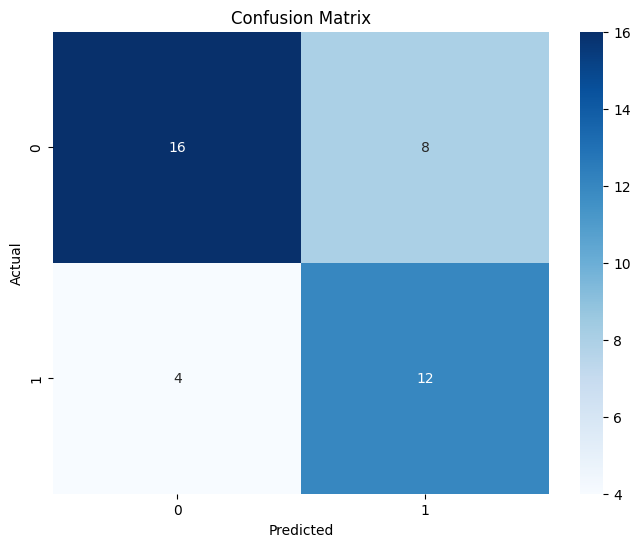
from sklearn.metrics import accuracy_score
# Assuming 'y' contains the true labels and 'pred2' contains the predicted labels
accuracy = accuracy_score(y, pred2)
print(f"Accuracy: {accuracy}")
Accuracy: 0.7
|
6.4 Evaluation and comparison of a classification model
6.4.1 Evaluation of a classification model
Suppose there are two groups \(\small G_1 , G_2\), and there are \(n\) number of data whose group affiliation is known.
As we discussed in section 6.1.1, if a classification model is used to classify each data,
the actual group of data and the group classified by the model can be compared and summarized in Table 6.4.1.
| Table 6.4.1 Table for the test results of the actual group and the classified group |
|
|
Classified group |
|
|
|
\(\small G_1\) |
\(\small G_2\) |
Total |
| Actual group |
\(\small G_1\) |
\(\small f_{11}\) |
\(\small f_{12}\) |
\(\small f_{11} + f_{12}\) |
| \(\small G_2\) |
\(\small f_{21}\) |
\(\small f_{22}\) |
\(\small f_{21} + f_{22}\) |
|
Total |
|
|
\(n\) |
Here, \(f_{ij}\) means the number of data of the group \(G_i\) classified into the group \(G_j\).
The number of data correctly classified out of the total data is \(f_{11} + f_{22}\), and the number of data
incorrectly classified is \(f_{12} + f_{21}\). As we defined in the section 6.1.1,
the
accuracy of the classification model is the ratio of the number of correctly classified data
out of the total number of data, and the
error rate is the ratio of the number of incorrectly classified data
out of the total number of data.
$$
\begin{align}
\text{Accuracy} &= \frac{f_{11} + f_{22}}{n} \\
\text{Error rate} &= \frac{f_{12} + f_{21}}{n}
\end{align}
$$
The accuracy and error rate can be considered reasonable measures if the risk of misclassification
of the group \(G_{1}\), \(f_{12}\), and the risk of misclassification of the group \(G_{2}\), \(f_{21}\),
are the same. However, in real problems, the risk of misclassification may be different for each group.
For example, consider two types of misclassification that a doctor misclassifies a cancer patient
as a healthy person and a doctor misclassifies a healthy person as a cancer patient.
The former case has a greater risk of misclassification than the latter because it carries the risk of shortening life.
When the risk of misclassification is different, the following measures called
sensitivity,
specificity, and
precision are used.
$$
\begin{align}
\text{Sensitivity} &= \frac{f_{11}}{f_{11} + f_{12}} \\
\text{Specificity} &= \frac{f_{22}}{f_{21} + f_{22}} \\
\text{Precision} &= \frac{f_{11}}{f_{11} + f_{21}}
\end{align}
$$
In the example above, sensitivity is the rate at which actual cancer patients are classified as cancer patients,
specificity is the rate at which healthy people are classified as healthy people, and precision is the rate
at which actual cancer patients are classified among classified as cancer patients. Accuracy can be expressed
as the weighted sum of sensitivity and specificity.
$$
\text{Accuracy} = \frac{f_{11} + f_{12}}{n} \text{(Sensitivity)} + \frac{f_{21} + f_{22}}{n} \text{(Specificity)}
$$
Lift chart, confusion matrix, expected profit and ROC curve are graphs that evaluate classification models
using sensitivity and specificity.
Lift Chart
Assume that the results of a classification model are expressed as continuous values, such as the posterior probability
of a Bayes classification model, and that a large posterior probability means a high probability of being classified
as group 1. Suppose we arrange all data in descending order of posterior probability and observe the top 10% of
the data. In that case, the rate of classifying the actual group 1, as group 1 will be very high if the classification model is good.
The rate of group 1 among the entire data is called the baseline response (%), and the sensitivity of classifying
actual group 1 as group 1 for the top 10% data is called the upper 10% response. The response rate of the top 10% data
compared to the baseline response rate is called the lift or improvement of the top 10%.
$$\it
\text{Top 10% lift} = \frac{\text{Response rate of top 10%}}{\text{Baseline response rate}}
$$
As a measure of the classification model, the lift is to compare how much the response rate of the top p%
of data has improved to the response rate of the entire data.
Example 6.4.1
Consider the naive Bayes classification model for the survey data in Example 6.3.3. The survey data
and their classification results with the posterior proability of each group are summarized in Table 6.4.2.
Find the lift table and draw lift chart.
| Table 6.4.2 Survey data and classification results with posterior probability of each group |
| Number |
Age |
Income
(unit USD) |
Credit |
Purchase |
Classification |
Posterior
Group 1: No |
Posterior
Group 2: Yes |
| 1 | 20s | LT2000 | Fair | Yes | No | 0.862 | 0.138 |
| 2 | 30s | GE2000 | Good | No | Yes | 0.165 | 0.835 |
| 3 | 20s | GE2000 | Fair | No | No | 0.806 | 0.194 |
| 4 | 20s | GE2000 | Fair | Yes | No | 0.806 | 0.194 |
| 5 | 20s | LT2000 | Bad | No | No | 1.000 | 0.000 |
| 6 | 30s | GE2000 | Fair | No | Yes | 0.409 | 0.591 |
| 7 | 30s | GE2000 | Good | Yes | Yes | 0.165 | 0.835 |
| 8 | 20s | LT2000 | Fair | No | No | 0.862 | 0.138 |
| 9 | 20s | GE2000 | Good | No | No | 0.542 | 0.458 |
| 10 | 30s | GE2000 | Fair | Yes | Yes | 0.409 | 0.591 |
| 11 | 30s | GE2000 | Good | Yes | Yes | 0.165 | 0.835 |
| 12 | 20s | LT2000 | Fair | No | No | 0.862 | 0.138 |
| 13 | 30s | GE2000 | Fair | No | Yes | 0.409 | 0.591 |
| 14 | 30s | LT2000 | Fair | Yes | No | 0.509 | 0.491 |
| 15 | 30s | GE2000 | Good | Yes | Yes | 0.165 | 0.835 |
| 16 | 30s | GE2000 | Fair | No | Yes | 0.409 | 0.591 |
| 17 | 20s | GE2000 | Bad | No | No | 1.000 | 0.000 |
| 18 | 20s | GE2000 | Bad | No | No | 1.000 | 0.000 |
| 19 | 30s | GE2000 | Good | Yes | Yes | 0.165 | 0.835 |
| 20 | 20s | LT2000 | Fair | No | No | 0.862 | 0.138 |
Answer
In order to make the lift table, we need first to arrange all data in descending order of the 1st group posterior probability,
and then organize them into 10 data categories (2 data each category is 10%). Since there are 12 data in group 1
and 8 data in group 2 out of the total 20 data, the baseline response rate of this data is
\(\frac{12}{20}\) which is 60%. In each data category, the number of the 1st group data, the cumulated
number of data, and the cumulated number of the 1st group data are counted to calculate the response rate,
cumulated response rate, and lift of each category. The captured column is the ratio of the number of
the 1st group out of the number of data in each category. The % response and Lift of the 1st category
which is the upper 10% of data are calculated as follows.
$$ \small
\begin{align}
\text{upper 10% Response} &= \frac{\text{Number of 1st group classified as group 1 in upper 10%}}{\text{Number of data in upper 10%}} \times 100 \\
\text{upper 10% Lift} &= \frac{\text{upper 10% Response}}{\text{Baseline response}} \times 100 \\
\end{align}
$$
Table 6.4.3 is the lift table and, and the lift chart is as in <Figure 6.4.1>.
| Table 6.4.3 Lift table for training data using the data in Table 6.4.2 |
Category
upper % |
Number of data |
Number of 1st group |
Cumulated num. of data |
Cumulated num. of 1st group |
Captured |
Response |
Cumulated response |
Lift |
| upper (0,10%] | 2 | 2 | 2 | 2 | 1.0 | 1.00 | 1.00 | 1.67 |
| (10,20%] | 2 | 2 | 4 | 4 | 1.0 | 1.00 | 1.00 | 1.67 |
| (20,30%] | 2 | 1 | 6 | 5 | 0.5 | 0.50 | 0.83 | 0.83 |
| (30,40%] | 2 | 2 | 8 | 7 | 1.0 | 1.00 | 0.88 | 1.67 |
| (40,50%] | 2 | 1 | 10 | 8 | 0.5 | 0.50 | 0.80 | 0.83 |
| (50,60%] | 2 | 1 | 12 | 9 | 0.5 | 0.50 | 0.75 | 0.83 |
| (60,70%] | 2 | 2 | 14 | 11 | 1.0 | 1.00 | 0.79 | 1.67 |
| (70,80%] | 2 | 0 | 16 | 11 | 0.0 | 0.00 | 0.69 | 0.00 |
| (80,90%] | 2 | 1 | 18 | 12 | 0.5 | 0.50 | 0.67 | 0.83 |
| (90,100%] | 2 | 0 | 20 | 12 | 0.0 | 0.00 | 0.60 | 0.00 |
<Figure 6.4.1> is a chart using the lift table in Table 6.4.3. The upper percentile of
of the data is on the x-axis, and the response rate, which is the rate of actually group 1 when the data
corresponding to the upper percentile category are considered as group 1, is plotted on the y-axis.
<Figure 6.4.1> Lift chart for training data
Since there is a small number of data in this example, we cannot see a general pattern of response rate.
In general, response rates show a decreasing pattern by upper % categories and a response rate becomes
below of the baseline response at one upper % category. We can also observe a category which the lift
becomes below 1. This upper % category can be used which value of the posterior probability will be
the boundary to decide a group. A lift chart is also drawn for both training and test data, which is called
a cross-lift chart. If it is a stable classification model, the lift charts of the training and test data
should not be significantly different.
We can use a lift chart to compare two classification models as shown in <Figure 6.4.2>.
Model \(\small M_1\) classifies group 1 more accurately than model \(\small M_2\) at each percentile of data,
so model \(\small M_1\) can be said to be better than \(\small M_2\).
<Figure 6.4.2> An example of a lift chart for comparing two classification models
Confusion matrix
The lift table sorts the entire data in descending order of posterior probability, divides them into
several categories with similar numbers of data, and then shows the response rate, lift, of each category of data.
The confusion matrix divides the posterior probability values into several cut-off values,
and then shows the correct classification, misclassification, accuracy, sensitivity, and specificity
of the entire data for each cut-off value. The confusion matrix is often used to determine
the cut-off value of the posterior probability to determine the group. Generally, the cut-off value
for determining the group is mainly accuracy, but sensitivity and specificity should also be carefully examined.
Example 6.4.2
Consider the naive Bayes classification model for the survey data in Example 6.3.3. The survey data
and their classification results with the posterior proability of each group are summarized in Table 6.4.2.
Find the confusion matrix and draw a graph of sensitivity, specificity and accuracy for each category of
posterior probability.
Answer
Consider a classification table created by dividing the posterior probability value into 0.1 units by
the cut-off value. For each cut-off value, data smaller than this value are classified into group 2,
and data larger than this value are classified into group 1. Table 6.4.4 is the confusion matrix
which shows the correct classification, misclassification, accuracy, sensitivity, and specificity of
the entire data for each cut-off value. <Figure 6.4.3> is the confusion matrix graph.
| Table 6.4.4 Confusion matrix |
| Number |
Posterior probability |
Number of data |
f11 |
f12 |
f21 |
f22 |
Accuracy |
Sensitivity |
Specificity |
| 1 | 0.00 | 20 | 12 | 0 | 8 | 0 | 0.600 | 1.000 | 0.000 |
| 2 | 0.10 | 20 | 12 | 0 | 8 | 0 | 0.600 | 1.000 | 0.000 |
| 3 | 0.20 | 20 | 11 | 1 | 4 | 4 | 0.750 | 0.917 | 0.500 |
| 4 | 0.30 | 20 | 11 | 1 | 4 | 4 | 0.750 | 0.917 | 0.500 |
| 5 | 0.40 | 20 | 11 | 1 | 4 | 4 | 0.750 | 0.917 | 0.500 |
| 6 | 0.50 | 20 | 8 | 4 | 3 | 5 | 0.650 | 0.667 | 0.625 |
| 7 | 0.60 | 20 | 7 | 5 | 2 | 6 | 0.650 | 0.583 | 0.750 |
| 8 | 0.70 | 20 | 7 | 5 | 2 | 6 | 0.650 | 0.583 | 0.750 |
| 9 | 0.80 | 20 | 7 | 5 | 2 | 6 | 0.650 | 0.583 | 0.750 |
| 10 | 0.90 | 20 | 3 | 9 | 0 | 8 | 0.550 | 0.250 | 1.000 |
| 11 | 1.00 | 20 | 0 | 12 | 0 | 8 | 0.400 | 0.000 | 1.000 |
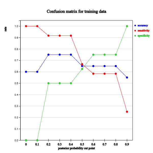
<Figure 6.4.3> Confusion matrix graph
ROC graph
When the result of a classification model can be expressed as a continuous value, such as the
posterior probability of a Bayes classification model or a logistic regression model, a
receiver operating
characteristic (ROC) graph can be drawn. The ROC graph is a graph with (1 - specificity) of
a classification model on the x-axis and sensitivity on the y-axis. It can be said that
the sensitivity is the true positive rate (TPR) and (1 - specificity) is the false positive rate (FPR)
which is the rate of misclassifying data from group 2 into group 1. A point on the ROC graph represents
the result of a classification model when a critical value of the posterior probability is used.
If we change the critical value, the classification result will be changed and a new point on the ROC graph
is created. In other words, the ROC graph examines the changes in FPR and TPR when the critical value of
the posterior probability is changged.
<Figure 6.4.4> is a ROC graph of two classification models, \(\small M_{1}\) and \(\small M_{2}\).
In the ROC graph, the point (FPR=0, TPR=0) represents a classification model that classifies all points
into group 2, the point (FPR=1, TPR=1) classifies all data into group 1, and the point (FPR=0, TPR=1)
represents an ideal model that does not misclassify group 2 data into group 1 and correctly classifies
all group 1 data. Therefore, a good classification model should have the classification results
located in the upper left corner of the ROC graph. The diagonal line in the figure shows an exceptional model
in which both the TPR and FPR ratios are the same, that means a special case in which data are randomly
classified into groups 1 and 2 with a fixed probability. In this case, group 1 data is classified into group 1
with probability \(p\) (TPR = \(p\)), and group 2 data is also classified into group 1 with probability
\(p\) (FPR = \(p\)). The ROC graph is helpful in comparing the performance of several classification models.
In <Figure 6.4.4>, the ROC graph of classification model \(\small M_{1}\) is located upper
on the left than that of classification model \(\small M_{2}\). This means that \(\small M_{1}\) has
the correct classification rate TPR is always better than the misclassification rate FPR for group 1,
so model \(\small M_{1}\) can be said to be better than model \(\small M_{2}\). In this case,
one classification model is always better than another classification model, but there are also cases
where the ROC graphs of the two models intersect so that neither model can always be said to be better.
<Figure 6.4.4> ROC graph for two classification models \(\small M_{1}\) and \(\small M_{2}\)
The area under the ROC graph is also called the
c-statistic, and it can be used to compare
how good the performance of the model is on average. In the case of an ideal model (FPR=0, TPR=1),
the area is 1, and in the case of a random classification where the classification result of
the model is located on the diagonal, the area is \(\frac{1}{2}\). If the area under the ROC graph
of one model is larger than that of another model, it can be said to be a better model on average.
To draw a ROC graph, first, sort in ascending order of the posterior probability of group 1 and
classify the entire data using each posterior probability value as the cut-off value for classifying
the two groups, calculate the sensitivity and specificity, and then draw a connecting line
using each sensitivity as the y-axis and (1 - specificity) as the x-axis. If you draw a ROC graph
in this way, the area under the curve, c-statistic, can be easily obtained. Let's look at the following
example to see how to draw a ROC graph.
Example 6.4.3
Consider the naive Bayes classification model for the survey data in Example 6.3.3. The survey data
and their classification results with the posterior proability of each group are summarized in Table 6.4.2.
The results are sorted in ascending order of the posterior probability of group 1.
Calculate TPR and FPR for ROC graph and draw the ROC graph of this classification model.
Answer
To draw a ROC graph, sort in ascending order of the posterior probability of group 1.
First, if we classify all data into group 1, the number of group 1 data classified into group 1 is
\(\small f_{11}\) = 12, and the number of group 2 data classified into group 1 is \(\small f_{21}\) = 8.
Next, if we classify the first data into group 2 and the second data and above into group 1,
we get \(\small f_{11}\) = 11, \(\small f_{12}\) = 1,\(\small f_{21}\) = 8. Next, if we classify
the first and second data into group 2 and the third data and above into group 1, we get
\(\small f_{11}\) = 11, \(\small f_{12}\) = 1,\(\small f_{21}\) = 7, \(\small f_{22}\) = 1.
If we classify in a similar way and obtain TPR and FPR, they are as shown in Table 6.4.5.
The rightmost column in the table is the case where all data is classified into group 2.
If you draw an ROC graph using the TPR and FPR in this table, it will look like <Figure 6.4.5>.
| Table 6.4.5 Calculation of TPR and FPR for ROC graph |
| Number |
Group |
Posterior probability |
f11 |
f12 |
f21 |
f22 |
TPR |
FPR |
| 0 | | | 12 | 0 | 8 | 0 | 1.000 | 1.000 |
| 1 | No | 0.165 | 11 | 1 | 8 | 0 | 0.917 | 1.000 |
| 2 | Yes | 0.165 | 11 | 1 | 7 | 1 | 0.917 | 0.875 |
| 3 | Yes | 0.165 | 11 | 1 | 6 | 2 | 0.917 | 0.750 |
| 4 | Yes | 0.165 | 11 | 1 | 5 | 3 | 0.917 | 0.625 |
| 5 | Yes | 0.165 | 11 | 1 | 4 | 4 | 0.917 | 0.500 |
| 6 | No | 0.409 | 10 | 2 | 4 | 4 | 0.833 | 0.500 |
| 7 | Yes | 0.409 | 10 | 2 | 3 | 5 | 0.833 | 0.375 |
| 8 | No | 0.409 | 9 | 3 | 3 | 5 | 0.750 | 0.375 |
| 9 | No | 0.409 | 8 | 4 | 3 | 5 | 0.667 | 0.375 |
| 10 | Yes | 0.509 | 8 | 4 | 2 | 6 | 0.667 | 0.250 |
| 11 | No | 0.542 | 7 | 5 | 2 | 6 | 0.583 | 0.250 |
| 12 | No | 0.806 | 6 | 6 | 2 | 6 | 0.500 | 0.250 |
| 13 | Yes | 0.806 | 6 | 6 | 1 | 7 | 0.500 | 0.125 |
| 14 | No | 0.862 | 5 | 7 | 1 | 7 | 0.417 | 0.125 |
| 15 | No | 0.862 | 4 | 8 | 1 | 7 | 0.333 | 0.125 |
| 16 | Yes | 0.862 | 4 | 8 | 0 | 8 | 0.333 | 0.000 |
| 17 | No | 0.862 | 3 | 9 | 0 | 8 | 0.250 | 0.000 |
| 18 | No | 1.000 | 2 | 10 | 0 | 8 | 0.167 | 0.000 |
| 19 | No | 1.000 | 1 | 11 | 0 | 8 | 0.083 | 0.000 |
| 20 | No | 1.000 | 0 | 12 | 0 | 3 | 0.000 | 0.000 |
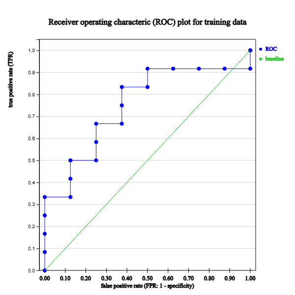
<Figure 6.4.5> ROC graph
6.4.2 Comparison of classification models
In order to classify data, rather than applying one classification model, several models are tried and the most appropriate model
for the given data is selected. The comparison of models is made using a comparison of accuracy, but the difference
in accuracy between the two models may not be statistically significant. In this section, we will look at the
confidence interval estimation for the accuracy of a classification model and the statistical method for
comparing the accuracy of two models.
In addition to accuracy, the comparison of two classification models should also consider the speed of processing
the algorithm on a computer, robustness for evaluating the impact of noisy data or missing values, scalability
for efficiently building the model even when a large amount of data is given, and interpretability of the model results.
Confidence interval for accuracy
Let \(p\) be the actual accuracy of the model and \(n\) be the number of test data set. If we let the random variable
\(\small X\) be the number of data correctly classified by the classification model, \(\small X\) is a binomial random
variable with parameters \(n\) and \(p\). In this case, the accuracy, \(\hat p = \frac{X}{n}\), of the classification experiment
has a mean of \(p\) and a variance of \(\frac{p(1-p)}{n}\). If \(n\) is sufficiently large,
the binomial distribution can be approximated by the normal distribution, so the 100(1-\(\alpha\))% confidence interval
for the actual accuracy \(p\) can be obtainable using the following probability statement.
$$
P ( - Z_{\frac{\alpha}{2}} < \frac{\hat p - p}{\sqrt{p(1-p)}} < Z_{\frac{\alpha}{2}} ) = 1 - \alpha
$$
Here, \( Z_{\frac{\alpha}{2}}\) means the right \(\frac{\alpha}{2}\) * 100% quantile of the standard normal distribution,
and when the confidence level is 95%, \( Z_{\frac{\alpha}{2}}\) = 1.96. If we rearrange this equation,
the confidence interval for the accuracy \(p\) can be shown as follows.
$$
\frac { ( 2 n \times \hat p + Z_{\frac{\alpha}{2}}^2 ) \; ± \; Z_{\frac{\alpha}{2}} \sqrt{ Z_{\frac{\alpha}{2}}^2 + 4 n \times \hat p - 4n \times {\hat p}^2 }} {2 n + 2 Z_{\frac{\alpha}{2}}^2}
$$
Example 6.4.4
When a classification model was applied to 100 test data, it had an accuracy of \(\hat p\) = 80%.
Estimate the confidence interval of actual accuracy with a 95% confidence level.
Answer
When the confidence level is 95%, \(\alpha\) = 0.05, so Z_{\frac{0.05}{2}} = 1.96.
The accuracy of the experiment \(\hat p\) = 0.8, and the number of data \(n\) = 100,
so by substituting the confidence interval formula, we get the following.
$$
\frac { ( 2 \times 100 \times 0.8 + {1.96}^2 ) \; ± \; 1.96 \sqrt{ {1.96}^2 + 4 \times 100 \times 0.8 - 4 \times 100 \times {0.8}^2 } }{2 \times 100 + 2 \times {1.96}^2}
$$
That is, the 95% confidence interval of the actual accuracy is (71.1%, 86.7%).
Comparison of accuracy of two models
Suppose that two classification models \( M_{1}\) and \( M_{1}\) are applied to two independent test data sets
of which their numbers of data are \(n_{1}\) and \(n_{2}\), and the accuracies \(\hat p_{1}\) and \(\hat p_{2}\) are measured
respectively. Let us find out how to test whether the accuracies \(\hat p_{1}\) and \(\hat p_{2}\) are statistically significant.
If \(n_{1}\) and \(n_{2}\) are sufficiently large, the accuracy \(\hat p_{1}\) and \(\hat p_{2}\) will approximately follow
normal distributions, and the difference in accuracy \(\hat p_{1} - \hat p_{2}\) will also approximately follow
a normal distribution with mean \( p_{1} - p_{2}\) and variance as follows.
$$
\frac{\hat p_{1} (1-\hat p_{1})}{n_1} + \frac{\hat p_{2} (1-\hat p_{2})}{n_2}
$$
Therefore, the (\(1 - \alpha\))% confidence interval of true accuracy difference, \(p_{1} - p_{2}\), is as follows.
$$
(\hat p_{1} - \hat p_{2}) \; ± \; Z_{\frac{\alpha}{2}} \; \sqrt{\frac{\hat p_{1} (1-\hat p_{1})}{n_1} + \frac{\hat p_{2} (1-\hat p_{2})}{n_2}}
$$
If this confidence interval includes 0, we can conclude that the accuracies of the two models are statistically the same.
Example 6.4.5
If a classification model \(\small M_{1}\) shows 85% accuracy on 50 test data and classification model \(\small M_{2}\)
shows 75% accuracy on 500 test data, can we conclude that classification model \(\small M_{1}\) is a better model than \(\small M_{2}\)?
Answer
The number of data applied to model \(\small M_{1}\) is \(\small n_{1}\) = 50 and the accuracy is \(\small \hat p_{1}\) = 0.85,
the number of data applied to model \(\small M_{2}\) is \(\small n_{2}\) = 500 and the accuracy is \(\small \hat p_{2}\) = 0.75,
Therefore, the 95% confidence interval is as follows.
\( \qquad
(0.85 - 0.75) \; ± \; 1.96 \sqrt{ \frac{ 0.85 (1-0.85)}{50} + \frac{ 0.75 (1-0.75)}{500}}
\)
\( \qquad
0.10 ± 1.96×0.0541
\)
Therefore, the 95% confidence interval is (-0.2060, 0.0060). This confidence interval includes 0,
so the difference in observed accuracy is not statistically significant. In other words, the true accuracies of model
\(\small M_{1}\) and model \(\small M_{2}\) are not statistically significant, so we cannot say
which classification model is better.
Generalized error considering model overfitting
A good classification model is a model that really classifies well when applied to actual data. However, a model
that shows satisfactory accuracy in test data may have poor classification accuracy when applied to actual data.
This case is called a model overfitting, and it often occurs in decision trees or neural network models.
There are various causes of overfitting, but it can occur when there is noisy data in the data or when the number of nodes
in the decision tree model is set too high. It can also occur when the training data, which is a part of the entire data set,
does not sufficiently represent the entire set. In order to prevent overfitting, the generalized error,
which is the sum of the experimental error of the model and the penalty term for the complexity of the model,
is used to compare and select a model among several models. For example, suppose that a decision tree \(T\) with \(k\) leaves
has an error rate at node \(t_{i}\), \(e(t_{i})\), when classifying \(n(t_{i})\) data. The generalized error
\(e_{g}(T)\) of this decision tree \(T\) can be defined as follows.
$$
\begin{align}
e_{g}(T) &= \frac{\sum_{i=1}^{k} [ e(t_{i}) + \Omega(t_{i}) ] }{\sum_{i=1}^{k} n(t_{i})} \\
&= \frac{e(T) + \Omega(T)}{\sum_{i=1}^{k} n(t_{i})}
\end{align}
$$
Here, \(\Omega(t_{i})\) is the penalty term in each node \(t_i\), \(e(T)\) is the overall error rate,
and \(\Omega(T)\) is the overall penalty term. If the penalty term of each node is \(\Omega(t_{i})\) = 0.2,
\(\Omega(T)\) becomes (the number of nodes) × 0.2, so the generalized error increases as the number of nodes increases.
Therefore, if there are two decision tree models with similar error rates, the generalization error of the model
with the smaller number of nodes is smaller.
6.5 Exercise
6.1 Ten data of two groups (+ group or - group) for two binary variables (A and B) are as follows.
| A |
B |
Group |
| T | F | + |
| T | T | + |
| T | T | + |
| T | F | - |
| T | T | + |
| F | F | - |
| F | F | + |
| F | F | - |
| T | T | + |
| T | F | - |
1) Calculate the information gain using the Gini coefficient for all ten data.
Calculate the information gain using the Gini coefficient for variable A and B.
Which variable's branching is better using these results in the decision tree?
2) Calculate the information gain using the entropy coefficient for all ten data.
Calculate the information gain using the entropy coefficient for variable A and B.
Which variable's branching is better using these results in the decision tree?
Compare the result with 1)
3) Find a decision tree using the entropy coefficient to classify the group.
When the values of variables A and B of a test data are T and F, respectively, classify the data using the decision tree.
4) Let the prior probability of the + group be 0.6 and the prior probability of the - group be 0.4.
Find a naive Bayes classification rule to classify the group.
When the values of variables A and B of a test data are T and F, respectively, classify the data using
the naive Bayes classification.
5) Find the lift chart, confusion matrix, and ROC curve in 4)
6.2 When we surveyed 20 people who visited a particular department store, 10 people made purchases,
and 10 people did not make purchases. The survey results of these 20 people's gender (M: male, F: female,
car ownership (S: small, M: medium, L: large), house ownership (Y: yes, N: no), and purchases (Y: yes, N: no) were as follows.
| Gender | Car | House | Purchase |
| M | M | N | Y |
| F | M | Y | N |
| F | L | Y | Y |
| F | L | Y | N |
| F | M | N | N |
| F | M | N | N |
| F | L | Y | Y |
| M | M | Y | Y |
| F | L | Y | N |
| M | L | N | Y |
| F | M | Y | Y |
| F | M | Y | N |
| M | M | N | N |
| F | M | N | Y |
| F | S | Y | N |
| F | S | N | N |
| M | S | N | Y |
| M | M | N | N |
| M | M | N | Y |
| M | S | N | N |
| F | L | Y | Y |
1) Find a decision tree using the entropy coefficient to classify the group.
When a customer is female, a large car owner, and has a house, classify the customer using the decision tree.
2) Let the prior probability of the purchasing group be 0.6 and the non-purchasing group be 0.4.
Find a naive Bayes classification rule to classify the group.
When a customer is female, a large car owner, and has a house, classify the customer using
the naive Bayes classification.
3) Find the lift chart, confusion matrix, and ROC curve in 2)