Chapter 8. Unsupervised Learning: Clustering Analysis
CHAPTER OBJECTIVES
The clustering analysis is a technique for finding clusters of data with similar properties when data
from multiple groups are mixed, and the group to which each data belongs is unknown.
We introduce the followings in this chapter.
• Basic concepts of clustering analysis and the evaluation methods of clustering models.
• Hierarchical clustering model, which has a long history, in section 8.2.
• \(\small K\)-means clustering model, which is frequently used in real practice, in section 8.3.
8.1 Basic concepts of clustering analysis
Classification analysis or supervised learning studied in Chapters 6 and 7 used data whose group affiliation
is known to obtain a classification function and then decided the data whose group affiliation
is unknown would be classified into which group using the classification function. However, when analyzing real data,
there is a need to classify data whose group affiliation is unknown into homogeneous groups, and
it is called
clustering analysis or
unsupervised learning. Clustering analysis can help understand
the structure of data (clustering for understanding) in situations where the content of the data is not well known,
or it can be a helpful starting point (clustering for utility) for other analyses by identifying the characteristics
of the formed clusters and the relationships between clusters. Clustering analysis is used in various fields,
such as psychology, biology, business administration, and information science.
Clustering analysis is a method of forming clusters based on the similarity or relationship between each data, such that
the data in a cluster are similar and the data in other clusters are different. At this time,
the higher the similarity within a cluster, the better, and the differences between clusters
should be as different as possible. However, it is generally difficult to define a cluster,
and it is unclear how many clusters to divide into. Many types of clustering analysis models have been developed
to apply to various types of data, but there is hardly a single clustering analysis model that is satisfactory
for all types of applications. Each clustering analysis model can show different performance when the data dimension
is low or high, when the data size is small or large, when the data density is small or high when there are
few or many outliers or extreme points, and when the data properties are discrete or continuous.
In general, after applying several clustering analysis models, an appropriate model is selected
based on the analyst's judgment.
In this chapter, we first introduce the hierarchical clustering model, which has been used for a long time.
Then, we introduce the \(\small K\)-means clustering, which is widely used.
Classification of clustering analysis models
Clustering analysis models are divided into hierarchical clustering models and partitional clustering models.
The
hierarchical clustering model allows subclusters within a cluster, and it groups the entire data into one cluster,
divides it into subclusters, and then divides each subcluster again. It can display the types of whole clusters
in a tree shape. Section 8.2 introduces hierarchical clustering models. The
partitional clustering model
is a method that divides the entire data without overlapping each other,
and Section 8.3 introduces the \(\small K\)-means clustering model.
Clustering analysis models can also be divided into exclusive clustering analysis, where one data must belong to one cluster,
and inclusive clustering analysis, where one data can belong to multiple clusters. The \(\small K\)-means clustering model
is an exclusive clustering analysis, and the fuzzy clustering model and the mixed distribution clustering model
are inclusive clustering analyses. The fuzzy cluster and mixed distribution clustering models indicate
the weight or probability that each data belongs to each cluster as a number between 0 and 1. However,
since the inclusive clustering analysis model generally classifies one data into a group with a higher probability,
the final data cluster can be an exclusive clustering analysis.
In addition, clustering analysis models are also classified into prototype-based models, density-based models,
and graph-based models.
The prototype-based model determines the form of the cluster based on how close the data is to the prototype
of each cluster, which has been determined in advance. The \(\small K\)-means clustering model is a prototype-based model.
In the case of continuous data, the cluster average is usually set as the prototype, and in the case of
discrete data, the mode of the cluster is used as the prototype. The density-based model is a method that
considers an area where data is distributed as a cluster when the density is very high. The graph-based model
is a method that considers each data as a node, connects the nodes based on a set distance, and then determines
the data corresponding to the connected nodes as a cluster. The Kohonen clustering model belongs to this.
Evaluation of clustering analysis models
The classification analysis model was created using training data, and then its accuracy was evaluated using test data.
However, evaluating which clustering analysis model is good is difficult, and the following factors are considered.
• Clustering tendency for a specific data set
• Number of accurate clusters
• Comparison of characteristics of formed clusters
Various measures can be considered for evaluating these factors, such as the response within a cluster,
cohesion and separation between clusters. In the case of clustering models
that utilize distance or similarity between data, the cohesion of cluster \(\small G_{i}\) and the separation
between two clusters \(\small G_{i}\) and \(\small G_{j}\) are defined as follows. Here,
\(\small d(\boldsymbol x, \boldsymbol y)\) is the distance between data \(\boldsymbol x\) and data \(\boldsymbol y\).
$$ \small
\begin{align}
\text{Cohesion} (G_{i}) &= \sum_{\boldsymbol x , \; \boldsymbol y \; \in \; G_{i}} \; d(\boldsymbol x, \boldsymbol y) \\
\text{Separation} (G_{i} , G_{j}) &= \sum_{\boldsymbol x \; \in \; G_{i}} \; \sum_{\boldsymbol x \; \in \; G_{j}} \; d(\boldsymbol x, \boldsymbol y)
\end{align}
$$
In the clustering model based on the prototype, the cohesion and separation are defined as follows when
the centroids of clusters \(\small G_{i}\) and clusters \(\small G_{j}\) are \(\small \boldsymbol c_{i}\) and
\(\small \boldsymbol c_{j}\), respectively.
$$ \small
\begin{align}
\text{Cohesion} (G_{i}) &= \sum_{\boldsymbol x \; \in \; G_{i}} \; d(\boldsymbol x, \boldsymbol c_{i} ) \\
\text{Separation} (G_{i} , G_{j}) &= d(\boldsymbol c_{i}, \boldsymbol c_{j})
\end{align}
$$
In the case of cohesion, if the distance \(d(\boldsymbol x, \boldsymbol c_{i} )\) between the data
\(\boldsymbol x \) of cluster and the center \(\boldsymbol c_{i} \) is defined as the squared Euclidean distance,
the cohesion of cluster \(\small G_{i}\) becomes the sum of squared error (SSE).
When there are \(\small K\) clusters and the number of data in cluster \(\small G_{i}\) is \(\small n_{i}\),
the cohesion of the entire clustering model is calculated as the weighted sum of the cohesion of each cluster,
and the weight value \(\small w_{i}\) can be \(\small n_{i}\), \(\small \frac{1}{n_{i}}\), or other various
measures depending on the situation.
$$ \small
\text{Cohesion of total model} = \sum_{i=1}^{K} \; w_{i} \times (\text{Cohesion of cluster} \; G_{i} )
$$
8.2 Hierachical clustering model
The
hierarchical clustering model is a widely used method with a long history, and there are two main approaches
to forming clusters. The
agglomerative method starts from one data and groups the closest clusters
in order. There are several variations depending on how the distance between clusters is defined.
The second is the
divisive method, which considers all data as one cluster and divides them in order
so that the final cluster becomes one data. There are several variations depending on which cluster is first divided and how it is divided. In this section, only the agglomerative hierarchical clustering model is introduced.
The result of hierarchical clustering is often displayed in a dendrogram similar to a tree, as shown
on <Figure 8.2.1>, which shows the relationship between clusters and subclusters and the order
in which clusters are formed. The subset plot displays the entire data as one set, as shown in
<Figure 8.2.2>, and displays each hierarchical cluster as a subset plot within this set.
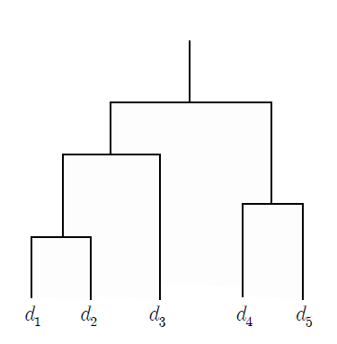
<Figure 8.2.1> Dendrogram for the results of hierarchical clustering
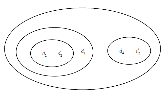
<Figure 8.2.2> Subset plot for the results of hierarchical clustering
Let \(n\) number of data observed for the \(m\) variables, \(\small \boldsymbol x =(x_{1}, x_{2}, ... x_{m})\),
be denoted as \(\small \boldsymbol x_{1}, \boldsymbol x_{2}, ... \boldsymbol x_{n}\).
The agglomerative hierarchical clustering algorithm first calculates the \(n\) × \(n\) distance matrix
or similarity matrix, \(D = \{ d_{ij} \}\), between all data where \( d_{ij} \) means the distance
between data \(\small \boldsymbol x_{i}\) and \(\small \boldsymbol x_{j}\).
$$
D = \left [ \matrix { d_{11} & d_{12} & ... & d_{1n} \cr d_{21} & d_{22} & ... & d_{2n} \cr ... & ... & ... & ... \cr d_{n1} & d_{n2} & ... & d_{nn} } \right ]
$$
After considering each data as a cluster, the two closest clusters are grouped into one cluster,
and the similarity matrix between this cluster and the remaining clusters is modified. At this time,
the similarity between clusters must be defined. The same method is repeated until the number of clusters
becomes one, which can be summarized as the following algorithm.
Agglomerative hierarchical clustering algorithm
| Step 1 |
Consider each data as one cluster and calculate the similarity matrix of all data.
|
| Step 2 |
repeat |
| Step 3 |
\(\qquad\)Group the two closest clusters into one cluster. |
| Step 4 |
\(\qquad\)Obtain the similarity matrix between all clusters including the newly formed cluster. |
| Step 5 |
until (the number of clusters becomes one) |
8.2.1 Method of linkage
The hierarchical clustering algorithm has several variations depending on how the distance between clusters is defined.
There are several methods for defining the distance between a cluster and other clusters: single linkage,
complete linkage, average linkage, median linkage, centroid linkage, and Ward method.
A. Single linkage
In the single linkage or shortest distance method, if the data with the closest distance in the
\(n\) × \(n\) distance matrix \(\small D = \{ d_{ij} \}\) are \(\small U\) and \(\small V\), the two data
are first grouped to form a cluster \(\small (UV)\).
The next step calculates the distance between cluster \(\small (UV)\) and the remaining \(n-2\) other data or clusters.
The single linkage distance between cluster \(\small (UV)\) and cluster \(\small W\) is calculated as follows:
$$
d_{(UV)W } = min ( d_{UW}, d_{VW} )
$$
In the modified distance matrix, the two data or clusters with the closest distance are combined into a new cluster.
Repeat this process until a single cluster includes all data.
Example 8.2.1
The five observed data for two variables \(\small x_{1}\) and \(\small x_{2}\) and the matrix of squared Euclid
distances between these data are as follows. Create a hierarchical cluster using the single linkage method.
| Table 8.2.1 Five observed data and the matrix of squared Euclid distances |
|
|
Distance/th>
|
| Data |
\(\small (x_{1}, \small x_{2})\) |
\(\small A\) |
\(\small B\) |
\(\small C\) |
\(\small D\) |
\(\small E\) |
| \(\small A\) | (1, 5) | 0 | |
| \(\small B\) | (2, 4) | 2 | 0 |
| \(\small C\) | (4, 6) | 10 | 8 | 0 |
| \(\small D\) | (4, 3) | 13 | 5 | 9 | 0 |
| \(\small E\) | (5, 3) | 20 | 10 | 10 | 1 | 0 |
Answer
Since the distance between data \(\small D\) and \(\small E\) is 1, which is the minimum, \(\small (DE)\) is the first cluster,
and the distance between cluster \(\small (DE)\) and the remaining data is calculated using the single linkage method,
and the distance matrix is modified as follows.
\( \small \qquad d((DE), A) = min(d(D,A), d(E,A)) = min(13, 20) = 13 \)
\( \small \qquad d((DE), B) = min(d(D,B), d(E,B)) = min(5, 10) = 5 \)
\( \small \qquad d((DE), C) = min(d(D,C), d(E,C)) = min(9, 10) = 9 \)
| Table 8.2.2 Modified distance matrix with cluster \(\small (DE)\) using the single linkage |
|
Distance/th>
|
| Cluster |
\(\small A\) |
\(\small B\) |
\(\small C\) |
\(\small (DE)\) |
| \(\small A\) | 0 | |
| \(\small B\) | 2 | 0 |
| \(\small C\) | 10 | 8 | 0 |
| \(\small (DE)\) | 13 | 5 | 9 | 0 |
Here, the minimum distance is \(\small d(A,B)\) = 2, so \(\small (AB)\) becomes the next cluster.
If we calculate the distance between clusters \(\small (AB)\) and \(\small C\) , \(\small (DE)\) using the
single linkage method and modify the distance matrix, we get the following.
\( \small \qquad d((AB), C) = min(d(A,C), d(B,C)) = min(10, 8) = 8 \)
\( \small \qquad d((AB), (DE)) = min(d(A, (DE)), d(B,(DE)) = min(13, 5) = 5 \)
| Table 8.2.3 Modified distance matrix with cluster \(\small (AB)\) using the single linkage |
|
Distance/th>
|
| Cluster |
\(\small (AB)\) |
\(\small C\) |
\(\small (DE)\) |
| \(\small (AB)\) | 0 | |
| \(\small C\) | 8 | 0 |
| \(\small (DE)\) | 5 | 9 | 0 |
Here, the minimum distance is \(\small (d(AB), (DE))\) = 5, so \(\small (AB)(DE)\) becomes the next cluster.
If we calculate the distance between clusters \(\small (AB)(DE)\) and \(\small C\) using the
single linkage method, we get the following.
\( \small \qquad d((AB)(DE), C) = min(d((AB), C), d((DE), C)) = min(8, 9) = 8 \)
If the above single linkage method is displayed as a dendrogram, it is as shown in <Figure 8.2.3>.
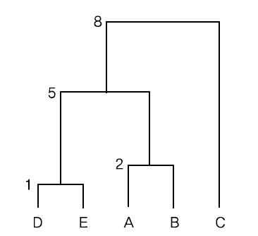
<Figure 8.2.3> Hierarchical clustering dendrogram using the single linkage
B. Complete linkage
In the complete linkage or maximum distance method, if the data with the closest distance in the
\(n\) × \(n\) distance matrix \(\small D = \{ d_{ij} \}\) are \(\small U\) and \(\small V\), the two data
are first grouped to form a cluster \(\small (UV)\).
The next step calculates the distance between cluster \(\small (UV)\) and the remaining \(n-2\) other data or clusters.
The complete linkage distance between cluster \(\small (UV)\) and cluster \(\small W\) is calculated as follows:
$$
d_{(UV)W } = max ( d_{UW}, d_{VW} )
$$
In the modified distance matrix, the two data or clusters with the closest distance are combined into a new cluster.
Repeat this process until a single cluster includes all data.
Example 8.2.2
The five observed data for two variables \(\small x_{1}\) and \(\small x_{2}\) and the matrix of squared Euclid
distances between these data are as follows. Create a hierarchical cluster using the complete linkage method.
| Table 8.2.4 Five observed data and the matrix of squared Euclid distances |
|
|
Distance/th>
|
| Data |
\(\small (x_{1}, \small x_{2})\) |
\(\small A\) |
\(\small B\) |
\(\small C\) |
\(\small D\) |
\(\small E\) |
| \(\small A\) | (1, 5) | 0 | |
| \(\small B\) | (2, 4) | 2 | 0 |
| \(\small C\) | (4, 6) | 10 | 8 | 0 |
| \(\small D\) | (4, 3) | 13 | 5 | 9 | 0 |
| \(\small E\) | (5, 3) | 20 | 10 | 10 | 1 | 0 |
Answer
Since the distance between data \(\small D\) and \(\small E\) is 1, which is the minimum, \(\small (DE)\) is the first cluster,
and the distance between cluster \(\small (DE)\) and the remaining data is calculated using the complete linkage method,
and the distance matrix is modified as follows.
\( \small \qquad d((DE), A) = max(d(D,A), d(E,A)) = max(13, 20) = 20 \)
\( \small \qquad d((DE), B) = max(d(D,B), d(E,B)) = max(5, 10) = 10 \)
\( \small \qquad d((DE), C) = max(d(D,C), d(E,C)) = max(9, 10) = 10 \)
| Table 8.2.5 Modified distance matrix with cluster \(\small (DE)\) using the complete linkage |
|
Distance/th>
|
| Cluster |
\(\small A\) |
\(\small B\) |
\(\small C\) |
\(\small (DE)\) |
| \(\small A\) | 0 | |
| \(\small B\) | 2 | 0 |
| \(\small C\) | 10 | 8 | 0 |
| \(\small (DE)\) | 20 | 10 | 10 | 0 |
Here, the minimum distance is \(\small d(A,B)\) = 2, so \(\small (AB)\) becomes the next cluster.
If we calculate the distance between clusters \(\small (AB)\) and \(\small C\) , \(\small (DE)\) using the
complete linkage method and modify the distance matrix, we get the following.
\( \small \qquad d((AB), C) = max(d(A,C), d(B,C)) = max(10, 8) = 10 \)
\( \small \qquad d((AB), (DE)) = max(d(A, (DE)), d(B,(DE)) = max(20, 10) = 20 \)
| Table 8.2.6 Modified distance matrix with cluster \(\small (AB)\) using the complete linkage |
|
Distance |
| Cluster |
\(\small (AB)\) |
\(\small C\) |
\(\small (DE)\) |
| \(\small (AB)\) | 0 | |
| \(\small C\) | 10 | 0 |
| \(\small (DE)\) | 20 | 10 | 0 |
Here, the minimum distance is \(\small d((AB), C)\) = \(\small d(C, (DE))\) = 10, so
\(\small (AB)C\) or \(\small C(DE)\) becomes the next cluster. Let's select \(\small C(DE)\) is the next cluster.
If we calculate the distance between clusters \(\small (AB)\) using the
complete linkage method, we get the following.
\( \small \qquad d((AB), C(DE)) = max(d((AB), C), d((AB), (DE))) = max(10, 20) = 20 \)
If the above complete linkage method is displayed as a dendrogram, it is as shown in <Figure 8.2.4>.
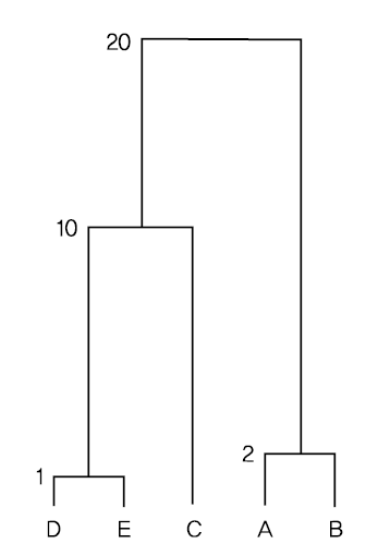
<Figure 8.2.4> Hierarchical clustering dendrogram using the complete linkage
C. Average linkage
In the average linkage method, if the data with the closest distance in the
\(n\) × \(n\) distance matrix \(\small D = \{ d_{ij} \}\) are \(\small U\) and \(\small V\), the two data
are first grouped to form a cluster \(\small (UV)\).
The next step calculates the average distance between cluster \(\small (UV)\) and the other cluster
\(\small W\) as follows.
$$
d_{(UV)W } = \frac{\sum_{\boldsymbol x_{i} \in (UV)} \sum_{\boldsymbol x_{j} \in W} \; d(\boldsymbol x_{i}, \boldsymbol x_{j}) }{n_{(UV)} \times n_{W}}
$$
Here \( \small d(\boldsymbol x_{i}, \boldsymbol x_{j}) \) is the distance between the data
\( \small \boldsymbol x_{i} \) in the cluster \(\small (UV)\) and the data \( \small \boldsymbol x_{j} \)
in the cluster \( \small W\), and \( n_{(UV)}\) and \( n_{W}\) are the number of data
in the cluster \(\small (UV)\) and \( \small W\) respectively.
In the modified distance matrix, the two data or clusters with the closest distance are combined into a new cluster.
Repeat this process until a single cluster includes all data.
Example 8.2.3
The five observed data for two variables \(\small x_{1}\) and \(\small x_{2}\) and the matrix of squared Euclid
distances between these data are as follows. Create a hierarchical cluster using the average linkage method.
| Table 8.2.7 Five observed data and the matrix of squared Euclid distances |
|
|
Distance/th>
|
| Data |
\(\small (x_{1}, \small x_{2})\) |
\(\small A\) |
\(\small B\) |
\(\small C\) |
\(\small D\) |
\(\small E\) |
| \(\small A\) | (1, 5) | 0 | |
| \(\small B\) | (2, 4) | 2 | 0 |
| \(\small C\) | (4, 6) | 10 | 8 | 0 |
| \(\small D\) | (4, 3) | 13 | 5 | 9 | 0 |
| \(\small E\) | (5, 3) | 20 | 10 | 10 | 1 | 0 |
Answer
Since the distance between data \(\small D\) and \(\small E\) is 1, which is the minimum, \(\small (DE)\) is the first cluster,
and the distance between cluster \(\small (DE)\) and the remaining data is calculated using the average linkage method,
and the distance matrix is modified as follows.
\( \small \qquad d((DE), A) = \frac{d(D,A) + d(E,A)}{2 \times 1} = \frac {13 + 20}{2} = 16.5 \)
\( \small \qquad d((DE), B) = \frac{d(D,B) + d(E,B)}{2 \times 1} = \frac {5 + 10}{2} = 7.5 \)
\( \small \qquad d((DE), C) = \frac{d(D,C) + d(E,C)}{2 \times 1} = \frac {9 + 10}{2} = 9.5 \)
| Table 8.2.8 Modified distance matrix with cluster \(\small (DE)\) using the single linkage |
|
Distance/th>
|
| Cluster |
\(\small A\) |
\(\small B\) |
\(\small C\) |
\(\small (DE)\) |
| \(\small A\) | 0 | |
| \(\small B\) | 2 | 0 |
| \(\small C\) | 10 | 8 | 0 |
| \(\small (DE)\) | 16.5 | 7.5 | 9.5 | 0 |
Here, the minimum distance is \(\small d(A,B)\) = 2, so \(\small (AB)\) becomes the next cluster.
If we calculate the distance between clusters \(\small (AB)\) and \(\small C\) , \(\small (DE)\) using the
average linkage method and modify the distance matrix, we get the following.
\( \small \qquad d((AB), C) = \frac{d(A,C) + d(B,C)}{2 \times 1} = \frac{10 + 8}{2} = 9 \)
\( \small \qquad d((AB), (DE)) = \frac{d(A,D) + d(A,E) + d(B,D) + d(B,E)}{2 \times 2} = \frac{13+20+5+10}{4} = 12 \)
| Table 8.2.9 Modified distance matrix with cluster \(\small (AB)\) using the average linkage |
|
Distance/th>
|
| Cluster |
\(\small (AB)\) |
\(\small C\) |
\(\small (DE)\) |
| \(\small (AB)\) | 0 | |
| \(\small C\) | 9 | 0 |
| \(\small (DE)\) | 12 | 9.5 | 0 |
Here, the minimum distance is \(\small (d(AB), C)\) = 9, so \(\small (AB)C\) becomes the next cluster.
If we calculate the distance between clusters \(\small (AB)C\) and \(\small (DE)\) using the
average linkage method, we get the following.
\( \small \qquad d((AB)C, (DE)) = \frac{d(A,D)+d(A,E)+d(B,D)+d(B,E)+d(C,D)+d(C,E)}{3 \times 2} = \frac{12+20+5+10+9+10}{6} = 11.1 \)
If the above average linkage method is displayed as a dendrogram in <Figure 8.2.5>.
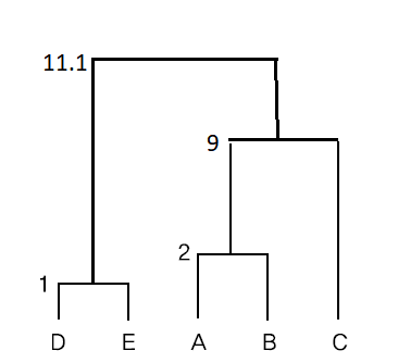
<Figure 8.2.5> Hierarchical clustering dendrogram using the average linkage
D. Centroid linkage
In the centroid linkage method, the distance between two clusters is calculated as the distance
between the centroids of the two clusters. If the number of data belonging to cluster \(\small G_{i}\) is
\(n_{i}\) and the centroid of the cluster is \(\boldsymbol c_{i}\),
and the number of data belonging to cluster \(\small G_{j}\) is
\(n_{j}\) and the centroid of the cluster is \(\boldsymbol c_{j}\), then the distance between two clusters,
\(\small d(G{i}, G_{j}) \), is defined as the squared Euclid distance between the two centroids as follows.
$$ \small
d(G{i}, G_{j}) = ||\boldsymbol c_{i} - \boldsymbol c_{j} ||^{2}
$$
If two clusters are combined, the center of the new cluster, \(\boldsymbol c\), is calculated
using the weighted average as follows.
$$ \small
\boldsymbol c = \frac{n_{i} \boldsymbol c_{i} + n_{j} \boldsymbol c_{j}}{n_{i} + n_{j}}
$$
After calculating the distance between each cluster, a new cluster is formed with the data with
the closest centroid distance.
Repeat this process until a single cluster includes all data.
Example 8.2.4
The five observed data for two variables \(\small x_{1}\) and \(\small x_{2}\) and the matrix of squared Euclid
distances between these data are as follows. Create a hierarchical cluster using the single linkage method.
| Table 8.2.10 Five observed data and the matrix of squared Euclid distances |
|
|
Distance/th>
|
| Data |
\(\small (x_{1}, \small x_{2})\) |
\(\small A\) |
\(\small B\) |
\(\small C\) |
\(\small D\) |
\(\small E\) |
| \(\small A\) | (1, 5) | 0 | |
| \(\small B\) | (2, 4) | 2 | 0 |
| \(\small C\) | (4, 6) | 10 | 8 | 0 |
| \(\small D\) | (4, 3) | 13 | 5 | 9 | 0 |
| \(\small E\) | (5, 3) | 20 | 10 | 10 | 1 | 0 |
Answer
Since the distance between data \(\small D\) and \(\small E\) is 1, which is the minimum, \(\small (DE)\) is the first cluster,
and the distance between cluster \(\small (DE)\) and the remaining data is calculated using the centroid linkage method,
and the distance matrix is modified as follows.
\( \small \qquad d((DE), A) = (4.5 - 1)^2 + (3-5)^2 = 16.25 \)
\( \small \qquad d((DE), B) = (4.5 - 2)^2 + (3-4)^2 = 7.25 \)
\( \small \qquad d((DE), C) = (4.5 - 4)^2 + (3-6)^2 = 9.25 \)
| Table 8.2.11 Modified distance matrix with cluster \(\small (DE)\) using the centroid linkage |
|
Distance/th>
|
| Cluster |
\(\small A\) |
\(\small B\) |
\(\small C\) |
\(\small (DE)\) |
| \(\small A\) | 0 | |
| \(\small B\) | 2 | 0 |
| \(\small C\) | 10 | 8 | 0 |
| \(\small (DE)\) | 16.25 | 7.25 | 9.25 | 0 |
Here, the minimum distance is \(\small d(A,B)\) = 2, so \(\small (AB)\) becomes the next cluster and
the center of the cluster is \(\small \frac{(4,3) + (5,3)}{2} = (4.5, 3)\).
If we calculate the distance between clusters \(\small (AB)\) and \(\small C\) , \(\small (DE)\) using the
centroid linkage method and modify the distance matrix, we get the following.
\( \small \qquad d((AB), C) = (1.5 - 4)^2 + (4.5 - 6)^2 = 8.5 \)
\( \small \qquad d((AB), (DE)) = (1.5 - 4.5)^2 + (4.5 - 3)^2 = 11.25 \)
| Table 8.2.12 Modified distance matrix with cluster \(\small (AB)\) using the centroid linkage |
|
Distance/th>
|
| Cluster |
\(\small (AB)\) |
\(\small C\) |
\(\small (DE)\) |
| \(\small (AB)\) | 0 | |
| \(\small C\) | 8.5 | 0 |
| \(\small (DE)\) | 11.25 | 9.5 | 0 |
Here, the minimum distance is \(\small (d(AB), C))\) = 8.5, so \(\small (AB)C\) becomes the next cluster
and the center of the cluster is as follows.
\( \qquad \frac{2 \times (1.5, \; 4.5) + 1 \times (4, \; 6)}{2 + 1} \) = (2.3, 5)
If we calculate the distance between clusters \(\small (AB)C\) and \(\small (DE)\) using the
centroid linkage method, we get the following.
\( \small \qquad d((AB)C, (DE)) = (2.3 - 4.5)^2 + (5-3)^2 \) = 8.84
If the above centroid linkage method is displayed as a dendrogram as shown in <Figure 8.2.6>.
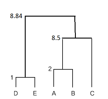
<Figure 8.2.6> Hierarchical clustering dendrogram using the centroid linkage
E. Ward linkage
The
Ward linkage is a method of merging clusters based on the within-group sum of squares rather than
linking data based on the distance between clusters. Ward linkage measures the information loss caused by grouping data
into a single cluster at each stage of clustering analysis by the cluster mean and the error sum of squares (\(\small ESS\))
between the data. If there are \(\small K\) clusters at the current stage in data with \(m\) variables
and \(n_{i}\) data in each cluster, the error sum of squares \(\small ESS_{i}\) of each cluster and
\(\small ESS\) of the entire cluster are as follows. Here, \(\small x_{ijk}\) is the measurement value
for the \(i\)-th variable of the \(j\)-th data of cluster \(\small G_{i}\), and
\( \small {\overline x}_{ik} = \frac {\sum_{j=1}^{n_{i}} \; x_{ijk} }{n_{i}} \)
means the mean value of variable \(k\) in cluster \(\small G_{i}\).
\( \small \qquad ESS_{i} = \sum_{j=1}^{n_{i}} \; \sum_{k=1}^{m} \; (x_{ijk} - \overline x_{ik} )^2 \)
\( \small \qquad ESS = \sum_{i=1}^{K} \; ESS_{i} = \sum_{i=1}^{K} \; \sum_{j=1}^{n_{i}} \; \sum_{k=1}^{m} \; (x_{ijk} - \overline x_{ik} )^2 \)
First, each data itself forms a cluster, then, since \(ESS_{i}\) for all i, \(ESS\) = 0.
At each stage of creating a cluster, the merging of all possible pairs of clusters is considered, and
the clusters are merged to create a new cluster so that the increment of \(ESS\) (information loss) due to
the merging of two clusters is minimized. The increment of \(ESS\) that occurs when grouping two clusters
\(\small G_{i}\) and \(\small G_{j}\), whose sizes are \(n_{i}\) and \(n_{j}\) respectively, is as follows,
and the Ward linkage method defines this increment as the distance between the two clusters \(\small G_{i}\)
and \(\small G_{j}\).
$$ \small
\qquad d(G_{i}, G_{j}) = \frac{|| \boldsymbol c_{i} - \boldsymbol c_{j} ||^2 }{\frac{1}{n_{i}} + \frac{1}{n_{j}} }
$$
Here, \( \boldsymbol c_{i}\) and \( \boldsymbol c_{j} \) are the averages of two clusters \(\small G_{i}\)
and \(\small G_{j}\) respectively. This result differs from the centroid linkage method because
the Ward linkage weights the distance between clusters means when calculating the distance between clusters.
The Ward linkage method tends to merge clusters of similar size.
Example 8.2.5
The five observed data for two variables \(\small x_{1}\) and \(\small x_{2}\) and the matrix of squared Euclid
distances between these data are as follows. Create a hierarchical cluster using the Ward linkage method.
| Table 8.2.13 Five observed data and the matrix of squared Euclid distances |
|
|
Distance/th>
|
| Data |
\(\small (x_{1}, \small x_{2})\) |
\(\small A\) |
\(\small B\) |
\(\small C\) |
\(\small D\) |
\(\small E\) |
| \(\small A\) | (1, 5) | 0 | |
| \(\small B\) | (2, 4) | 2 | 0 |
| \(\small C\) | (4, 6) | 10 | 8 | 0 |
| \(\small D\) | (4, 3) | 13 | 5 | 9 | 0 |
| \(\small E\) | (5, 3) | 20 | 10 | 10 | 1 | 0 |
Answer
When each data is considered as a cluster, the increment of ESS is the squared Euclid distance. Since the distance
between data D and E is 1, which is the minimum, (DE) becomes the first cluster.
The center of the cluster (DE) is \( \frac{(4,3) + (5,3)}{2} \) = (4.5, 3), so the distance is calculated using
the Ward linkage method for the remaining data, and the distance matrix is modified as follows.
\( \small \qquad d((DE), A) = \frac{(4.5 - 1)^2 + (3 - 5)^2)}{\frac{1}{2} +\frac{1}{1}} = 11.17 \)
\( \small \qquad d((DE), B) = \frac{(4.5 - 2)^2 + (3 - 4)^2)}{\frac{1}{2} +\frac{1}{1}} = 4.83 \)
\( \small \qquad d((DE), C) = \frac{(4.5 - 4)^2 + (3 - 6)^2)}{\frac{1}{2} +\frac{1}{1}} = 6.17 \)
| Table 8.2.14 Modified distance matrix with cluster \(\small (DE)\) using the Ward linkage |
|
Distance/th>
|
| Cluster |
\(\small A\) |
\(\small B\) |
\(\small C\) |
\(\small (DE)\) |
| \(\small A\) | 0 | |
| \(\small B\) | 2 | 0 |
| \(\small C\) | 10 | 8 | 0 |
| \(\small (DE)\) | 11.17 | 4.83 | 6.17 | 0 |
Here, the minimum distance is \(\small d(A,B)\) = 2, so \(\small (AB)\) becomes the next cluster and the center
of the cluster becomes \( \frac{(1,5) + (2,4)}{2} \) = (1.5, 4.5).
If we calculate the distance between clusters \(\small (AB)\) and \(\small C\) , \(\small (DE)\) using the
Ward linkage method and modify the distance matrix, we get the following.
\( \small \qquad d((AB), C) = \frac{(1.5 - 4)^2 + (4.5 - 6)^2)}{\frac{1}{2} +\frac{1}{1}} = 5.67 \)
\( \small \qquad d((AB), (DE)) = \frac{(1.5 - 4.5)^2 + (4.5 - 3)^2)}{\frac{1}{2} +\frac{1}{1}} = 11.25 \)
| Table 8.2.15 Modified distance matrix with cluster \(\small (AB)\) using the Ward linkage |
|
Distance/th>
|
| Cluster |
\(\small (AB)\) |
\(\small C\) |
\(\small (DE)\) |
| \(\small (AB)\) | 0 | |
| \(\small C\) | 5.67 | 0 |
| \(\small (DE)\) | 11.25 | 6.17 | 0 |
Here, the minimum distance is \(\small (d(AB), C)\) = 5.67, so \(\small (AB)C\) becomes the next cluster
and the center of the cluster becomes \( \frac{2 \times (1.5, 4.5) + 1 \times (4, 6)}{2 + 1} \) = (2.3, 5).
If we calculate the distance between clusters \(\small (AB)C)\) and \(\small DE\) using the
Ward linkage method, we get the following.
\( \small \qquad d((AB)C, (DE)) = \frac{(2.3 - 4.5)^2 + (5 - 3)^2)}{\frac{1}{3} +\frac{1}{2}} = 10.61 \)
If the above Ward linkage method is displayed as a dendrogram, it is as shown in <Figure 8.2.7>.
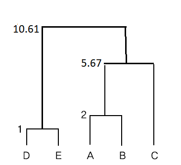
<Figure 8.2.7> Hierarchical clustering dendrogram using the Ward linkage
Hierarchical clustering module of 『eStatU』 using the 27 iris data is as follows. You can select clustering methods
discussed in this section, but it is limited up to 100 observations.
[Hierarchical clustering\
<Figure 8.2.8> Hierarchical clustering module in 『eStatU』
Characteristics of the hierarchical clustering model
The characteristics of the hierarchical clustering model are as follows.
1) The hierarchical clustering model is a method of finding a locally optimal cluster at each stage,
so it cannot be considered a general method of optimizing the entire objective function.
2) Once a cluster is created, the hierarchical clustering model does not consider the dissolution
of the created cluster at all in the next stage. The results of the hierarchical clustering model
are used as the initial clusters of the \(\small K\)-means clustering model in the next section
to test the stability of the results, etc.
3) When merging clusters in the average linkage method, centroid linkage method, and Ward linkage method,
the size of each cluster is weighted so that clusters with large sizes are merged if possible.
8.2.2 R and Python practice - Hierarchical clustering
You must install a package called
stats to use Hierarchical clustering using R.
From the main menu of R,
select ‘Package’ => ‘Install package(s)’, and a window called ‘CRAN mirror’ will appear. Here,
select ‘0-Cloud [https]’ and click ‘OK’. Then, when the window called ‘Packages’ appears, select
‘stats’ and click ‘OK’. dist() and hcluster() are used for the hierarchical clustering, and general usage and
key arguments of the functions are described in the following table.
Distance Matrix Computation
This function computes and returns the distance matrix computed by using the specified distance measure to compute the distances between the rows of a data matrix.
|
|
dist(x, method = "euclidean", diag = FALSE, upper = FALSE, p = 2)
|
| x |
a numeric matrix, data frame or "dist" object. |
| method |
the distance measure to be used. This must be one of "euclidean", "maximum", "manhattan", "canberra", "binary" or "minkowski". |
| diag |
logical value indicating whether the diagonal of the distance matrix should be printed by print.dist. |
| upper |
logical value indicating whether the upper triangle of the distance matrix should be printed by print.dist. |
| p |
The power of the Minkowski distance. |
| hclust {stats} |
Hierarchical Clustering
Hierarchical cluster analysis on a set of dissimilarities and methods for analyzing it.
|
|
hclust(d, method = "complete", members = NULL)
|
| d |
a dissimilarity structure as produced by dist. |
| members |
NULL or a vector with length size of d. |
An example of R commands for a Hierarchical clustering with 30 iris data is as follows.
| library(stats) |
| iris <- read.csv('http://estat.me/estat/Example/DataScience/Iris30.csv', header=T, as.is=FALSE) |
| attach(iris) |
# select Sepal.Length, Sepal.Width, Petal.Length, Petal.Width from iris data
iris4 <- iris[, c(2,3, 4, 5)]
|
# calculate distance matrix using squared Euclid distance
dist(iris4, method = 'euclidean')
|
| hclustIris4 <-hclust(distIris4, method = "ward.D") |
hclustIris4
Call: hclust(d = distIris4, method = "ward.D")
Cluster method   : ward.D
Distance         : euclidean
Number of objects: 30
|
# plot hierarchical clusters
plot(hclustIris4)
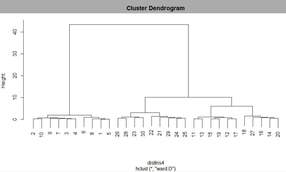
<Figure 8.2.8> Hierarchical clustering dendrogram using R
|
Python practice
[Colab]
# Import required libraries
import pandas as pd
import numpy as np
from scipy.cluster.hierarchy import dendrogram, linkage
from scipy.spatial.distance import pdist
import matplotlib.pyplot as plt
from sklearn.datasets import load_iris
# Load iris dataset
iris = load_iris()
iris_df = pd.DataFrame(data=iris.data, columns=iris.feature_names)
# Select the four features (equivalent to Sepal.Length, Sepal.Width, Petal.Length, Petal.Width)
iris4 = iris_df.iloc[:, [0, 1, 2, 3]]
# Calculate distance matrix using squared Euclidean distance
dist_matrix = pdist(iris4, metric='euclidean')
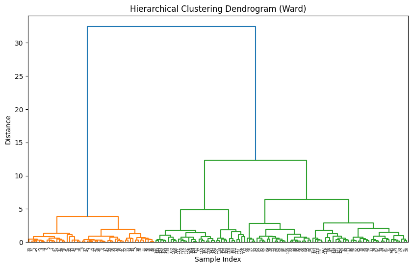
# Perform hierarchical clustering using Ward's method
hclust = linkage(dist_matrix, method='ward')
# Plot dendrogram
plt.figure(figsize=(10, 6))
dendrogram(hclust, labels=iris_df.index)
plt.title('Hierarchical Clustering Dendrogram (Ward)')
plt.xlabel('Sample Index')
plt.ylabel('Distance')
plt.show()
|
8.3 \(\small K\)-means clustering model
The
\(\small K\)-means clustering model is a prototype-based model, and if medians are used instead of means,
it is called
\(\small K\)-median clustering model. These models can be applied to continuous data,
and the mean and median of the data can be used as the centers of the clusters, respectively.
If there is no outlier, the \(\small K\)-means clustering model is frequently used.
A similar concept can be applied to discrete data by defining the centroid of the discrete data.
The clustering model requires an appropriate distance measure between data and a cluster.
\(\small K\)-means clustering model first determines the number of clusters \(\small K\)
and selects the initial center of each cluster. Then, each data is classified into a cluster with
the closest cluster center, and the center of each cluster is recalculated.
We can use the various distance measures studied in Chapter 2,
and in the case of continuous data, the Euclidean distance
is generally used. This method is repeated until there is no change in the cluster center. The basic procedure
of the \(\small K\)-means clustering model is summarized as follows.
\(\small K\)-means clustering algorithm
| Step 1 |
Determine the number of clusters \(\small K\) you want. |
| Step 2 |
Select the initial center of each cluster. |
| Step 3 |
repeat |
| Step 4 |
\(\qquad\)Classify each data into the cluster with the closest cluster center. |
| Step 5 |
\(\qquad\)Recalculate the center of each cluster. |
| Step 6 |
until (there is little change in the cluster center |
Example 8.3.1
For the two variables \(x_{1}\) and \(x_{2}\), four data were observed as follows. Find two clusters
using the 2-means clustering algorithm with the squared Euclid distance between the data.
| Table 8.3.1 Data for the 2-means clustering algorithm |
| Data |
(\(x_{1}, x_{2}\)) |
| A |
(3, 4) |
| B |
(-1, 2) |
| C |
(-2, -3) |
| D |
(1, -2) |
Answer
Let the center of cluster 1 be data A=(3,4) and the center of cluster 2 be data C=(-2,-3). The distances
from each data to the centers of the two clusters are as follows.
| Table 8.3.2 Distance between data and the center of cluster |
| Data |
Cluster 1
Distance to center (3, 4) |
Cluster 2
Distance to center (-2, -3) |
| A |
0 |
74 |
| B |
20 |
26 |
| C |
74 |
0 |
| D |
40 |
10 |
Therefore, if each data is classified by the nearest cluster center, data A and B are classified into cluster 1,
data C and D are classified into cluster 2, and the center of the new cluster 1 by the average is (1,3),
and the center of cluster 2 is (-0.5,-2.5). The distances from each data to the centers of the two new clusters are as follows.
| Table 8.3.3 Modified distance between data and the center of cluster |
| Data |
Cluster 1
Distance to center (1, 3) |
Cluster 2
Distance to center (-0.5, -2.5) |
| A |
5 |
54.5 |
| B |
5 |
20.5 |
| C |
45 |
2.5 |
| D |
25 |
2.5 |
If each data is classified by the nearest cluster center, data A and B are classified again as cluster 1,
and data C and D are classified as cluster 2, so the center of each cluster does not change, so the algorithm is stopped.
Finally, data A and B are classified as cluster 1, and data C and D are classified as cluster 2.
Theoretical background of the \(\small K\)-means clustering model
The hierarchical clustering model in Section 8.2 has a disadvantage: if data is assigned to a specific cluster,
it cannot be reassigned to another cluster. The \(\small K\)-means clustering model, on the other hand,
can assign the data to a different group in the next clustering stage.
Let's look at the theoretical background of the \(\small K\)-means clustering model.
Suppose there are \(m\) variables \(\small \boldsymbol x = (x_{1}, x_{2}, ... , x_{m}) \) and
\(n\) number of data observed for these variables. Let the \(\small K\) clusters be \(\small G_{1}, G_{2}, ... , G_{K}\),
the number of data observed in each cluster be \(\small n_{1}, n_{2}, ... , n_{K}\), and the mean of each cluster
be \(\small \boldsymbol c_{1}, \boldsymbol c_{2}, ... , \boldsymbol c_{K} \) as follows.
$$
\boldsymbol c_{i} = \frac{1}{n_{i}} \; \sum_{\boldsymbol x \in G_{i}} \; \boldsymbol x
$$
If \(\small d(\boldsymbol c_{i}, \boldsymbol x)\) is the distance between the center \(\small \boldsymbol c_{i}\) of cluster
\(\small G_{i}\) and the data \(\small \boldsymbol x\), the measure of cluster performance can be defined as
the sum of distances from all data to each center.
$$
\text{(Performance measure of clustering)} = \sum_{i=1}^{K} \; \sum_{\boldsymbol x \in G_{i}} \; d( \boldsymbol c_{i} , \boldsymbol x)
$$
When using the squared Euclid distance as a distance measure, the \(\small \boldsymbol c_{i}\)
that minimizes this performance measure of clustering can be shown to be the mean of the cluster.
Here, let us prove that \(\small \boldsymbol c_{i}\) is the cluster's mean when the data is only one-dimensional.
The performance measure of clustering is the following within sum of squares (WSS) in the case of the squared Euclid distance.
$$
\text{WSS} = \sum_{i=1}^{K} \; \sum_{x \in G_{i}} \; (c_{i} - x)^2
$$
In order to find \(\small c_{1}, c_{2}, ... , c_{K} \) that minimizes this WSS, we take partial differentiation
for each \(\small c_{i}, i=1,2, ... , K\), and set it to 0.
$$
\frac{\partial}{\partial c_{i}} \text{SSE} = \sum_{x \in G_{i}} \; 2 (c_{i} - x) = 0
$$
The solution to these simultaneous equations is as follows.
$$
c_{i} = \frac{1}{n_{i}} \; \sum_{x \in G_{i}} \; x
$$
That is, \(\small c_{1}, c_{2}, ... , c_{K} \) that minimize the SSE are each mean of the clusters.
If the data is one-dimensional and the absolute distance (Manhattan distance) is used as a distance measure,
the performance measure of clustering becomes the sum of absolute error (SAE) as follows.
$$
\text{SAE} = \sum_{i=1}^{K} \; \sum_{x \in G_{i}} \; | c_{i} - x |
$$
It can be shown that the solution \(\small c_{1}, c_{2}, ... , c_{K} \) that minimizes this SAE
are each median of the clusters. In general, the median is known to be less sensitive to extreme points or outliers.
Determine the number of cluster
In general, it is not easy to determine the number of clusters in \(\small K\)-means clustering model.
One method is first to examine the clustering results of the hierarchical clustering model in Section 8.2
and then decide the number of clusters. Another useful way is to analyze various \(\small K\) values and then compare
the within sum of squares. Selection of \(\small K\), which has the minimum within sum of squares is reasonable.
However, since the \(\small K\)-means clustering algorithm finds a solution that minimizes the within sum of squares,
this algorithm may find a local minimum rather than a global minimum. It is desirable to run the
initial center of each cluster as multiple data to prevent this problem and select a cluster with a smaller WSS.
\(\small K\)-means clustering module of 『eStatU』 provides a plot of the within sum of squares for various \(\small K\)
as follows. After selecting \(\small K\), you can do clustering analysis by checking 'fixed K'.
[\(\small K\)-means clustering]
<Figure 8.3.1> \(\small K\)-means clustering in 『eStatU』
In general, extreme points or outliers can seriously affect the \(\small K\)-means clustering model,
and we should try various distance measures. In other words, if there is an extreme point, the average of
that cluster is not suitable as a center measure for the cluster.
You can remove extreme points or outliers through exploratory data analysis to prevent this.
8.3.1 R and Python practice - \(\small K\)-means clustering
To use \(\small K\)-means clustering using R, you need to install a package called
stats.
From the main menu of R,
select ‘Package’ => ‘Install package(s)’, and a window called ‘CRAN mirror’ will appear.
Select ‘0-Cloud [https]’ and click ‘OK’. Then, when the window called ‘Packages’ appears, select
‘stats’ and click ‘OK’. The following table describes the function's general usage and key arguments.
\(\small K\)-Means Clustering
Perform k-means clustering on a data matrix.
|
|
kmeans(x, centers, iter.max = 10, nstart = 1, algorithm = c("Hartigan-Wong", "Lloyd", "Forgy", "MacQueen"), trace = FALSE)
|
| x |
numeric matrix of data, or an object that can be coerced to such a matrix (such as a numeric vector or a data frame with all numeric columns). |
| centers |
either the number of clusters, say k, or a set of initial (distinct) cluster centres. If a number, a random set of (distinct) rows in x is chosen as the initial centres. |
| test |
The data set for which we want to obtain the k-NN classification, i.e. the test set. |
| iter.max |
the maximum number of iterations allowed. |
| nstart |
if centers is a number, how many random sets should be chosen? |
An example of R commands for a \(\small K\)-means clustering with iris data when k = 3 is as follows.
| library(stats) |
| iris <- read.csv('http://estat.me/estat/Example/DataScience/Iris150.csv', header=T, as.is=FALSE) |
| attach(iris) |
# select Sepal.Length, Sepal.Width, Petal.Length, Petal.Width from iris data
iris4 <- iris[, c(2,3, 4, 5)]
|
| iriskmeans <- kmeans(iris4, centers = 3, iter.max = 1000) |
iriskmeans
K-means clustering with 3 clusters of sizes 38, 62, 50
Cluster means:
  Sepal.Length Sepal.Width Petal.Length Petal.Width
1     6.850000    3.073684     5.742105    2.071053
2     5.901613    2.748387     4.393548    1.433871
3     5.006000    3.428000     1.462000    0.246000
Clustering vector:
  [1] 3 3 3 3 3 3 3 3 3 3 3 3 3 3 3 3 3 3 3 3 3 3 3 3 3 3 3 3 3 3 3 3 3 3 3 3 3
 [38] 3 3 3 3 3 3 3 3 3 3 3 3 3 2 2 1 2 2 2 2 2 2 2 2 2 2 2 2 2 2 2 2 2 2 2 2 2
 [75] 2 2 2 1 2 2 2 2 2 2 2 2 2 2 2 2 2 2 2 2 2 2 2 2 2 2 1 2 1 1 1 1 2 1 1 1 1
[112] 1 1 2 2 1 1 1 1 2 1 2 1 2 1 1 2 2 1 1 1 1 1 2 1 1 1 1 2 1 1 1 2 1 1 1 2 1
[149] 1 2

Within cluster sum of squares by cluster:
[1] 23.87947 39.82097 15.15100
 (between_SS / total_SS =  88.4 %)
Available components:
[1] "cluster"      "centers"      "totss"        "withinss"     "tot.withinss"
[6] "betweenss"    "size"         "iter"         "ifault"
|
# the cluster vector only can be seen as follows.
1: verginica, 2: versicolor, 3: setosa
iriskmeans$cluster
  [1] 3 3 3 3 3 3 3 3 3 3 3 3 3 3 3 3 3 3 3 3 3 3 3 3 3 3 3 3 3 3 3 3 3 3 3 3 3
 [38] 3 3 3 3 3 3 3 3 3 3 3 3 3 2 2 1 2 2 2 2 2 2 2 2 2 2 2 2 2 2 2 2 2 2 2 2 2
 [75] 2 2 2 1 2 2 2 2 2 2 2 2 2 2 2 2 2 2 2 2 2 2 2 2 2 2 1 2 1 1 1 1 2 1 1 1 1
[112] 1 1 2 2 1 1 1 1 2 1 2 1 2 1 1 2 2 1 1 1 1 1 2 1 1 1 1 2 1 1 1 2 1 1 1 2 1
[149] 1 2
|
To make a classification cross table, you can use a vector of Species and iriskmeans$cluster which is the cluster
with table command as below. 'Setosa's are clustered 100% correctly, 'versicolor's are 48/50, but 'virginica's
are 36/50.
# 1: verginica, 2: versicolor, 3: setosa
classtable <- table(Species, iriskmeans$cluster)
Species       1  2  3
  setosa      0  0 50
  versicolor  2 48  0
  virginica  36 14  0
|
Python practice
[Colab]
# Import required libraries
import pandas as pd
import numpy as np
from sklearn.datasets import load_iris
from sklearn.cluster import KMeans
# Load iris dataset
iris = load_iris()
iris_df = pd.DataFrame(data=iris.data, columns=iris.feature_names)
iris_df['Species'] = pd.Categorical.from_codes(iris.target, iris.target_names)
# Select the four features (Sepal Length, Sepal Width, Petal Length, Petal Width)
iris4 = iris_df.iloc[:, [0, 1, 2, 3]]
# Perform k-means clustering
kmeans = KMeans(n_clusters=3, max_iter=1000, random_state=123)
iriskmeans = kmeans.fit(iris4)
# Get cluster assignments
cluster_labels = iriskmeans.labels_
# Print k-means resultsv
print("K-means clustering results:")
print(f"Cluster centers:\n{iriskmeans.cluster_centers_}")
print(f"Cluster assignments:\n{cluster_labels}")
# Create classification table (cross-tabulation of Species and clusters)
classtable = pd.crosstab(iris_df['Species'], cluster_labels,
rownames=['Species'], colnames=['Cluster'])
print("\nClassification table:")
print(classtable)
K-means clustering results:
Cluster centers:
[[6.85       3.07368421 5.74210526 2.07105263]
 [5.006      3.428      1.462      0.246     ]
 [5.9016129  2.7483871  4.39354839 1.43387097]]
Cluster assignments:
[1 1 1 1 1 1 1 1 1 1 1 1 1 1 1 1 1 1 1 1 1 1 1 1 1 1 1 1 1 1 1 1 1 1 1 1 1
 1 1 1 1 1 1 1 1 1 1 1 1 1 2 2 0 2 2 2 2 2 2 2 2 2 2 2 2 2 2 2 2 2 2 2 2 2
 2 2 2 0 2 2 2 2 2 2 2 2 2 2 2 2 2 2 2 2 2 2 2 2 2 2 0 2 0 0 0 0 2 0 0 0 0
 0 0 2 2 0 0 0 0 2 0 2 0 2 0 0 2 2 0 0 0 0 0 2 0 0 0 0 2 0 0 0 2 0 0 0 2 0
 0 2]

Classification table:
Cluster      0   1   2
Species
setosa       0  50   0
versicolor   2   0  48
virginica   36   0  14
|
8.4 Exercise
8.1 The distance matrix for five data (A, B, C, D, E) is as follows.
| Distance | A | B | C | D | E |
| A | 0 | | | | |
| B | 10 | 0 | | | |
| C | 41 | 64 | 0 | | |
| D | 55 | 47 | 44 | 0 | |
| E | 35 | 98 | 85 | 76 | 0 |
1) Create a hierarchical cluster using the single linkage method.
2) Create a hierarchical cluster using the complete linkage method.
3) Create a hierarchical cluster using the average linkage method.
4) Create a hierarchical cluster using the centroid linkage method.
5) Create a hierarchical cluster using the Ward linkage method.
8.2 The following six data were observed for two variables \(X_1\) and \(X_2\).
| Data | \(X_1\) | \(X_2\) |
| A | 3 | 4 |
| B | -1 | 2 |
| C | -2 | -3 |
| D | 1 | -2 |
| E | 1 | 3 |
| E | -1 | 2 |
1) Calculate the distance between the data using the Euclidean square distance.
Create a hierarchical cluster using the single linkage method.
2) Create a hierarchical cluster using the complete linkage method.
3) Create a hierarchical cluster using the average linkage method.
4) Create a hierarchical cluster using the centroid linkage method.
5) Create a hierarchical cluster using the Ward linkage method.
8.3 Create clusters using the 2-mean clustering model.
Use the mean as the central measure in the data of Problem 2.