Chapter 12. Correlation and Regression Analysis
[book] [eStat YouTube Channel]
- 12.1 Correlation Analysis
- 12.2 Simple Linear Regression Analysis
- 12.3 Multiple Linear Regression Analysis
- 12.4 Exercise
CHAPTER OBJECTIVES
From Chapter 7 to Chapter 10, we discussed the estimation and the testing hypothesis of parameters such as population mean and variance for single variable. This chapter describes a correlation analysis for two or more variables.If variables are related with each other, then a regression analysis is described to see how this association can be used. Simple linear regression analysis and multiple regression analysis are discussed.
12.1 Correlation Analysis
[presentation] [video]
Example 12.1.1 Based on the survey of advertising costs and sales for 10 companies that make the same product, we obtained the following data as in Table 12.1.1. Using 『eStat』 , draw a scatter plot for this data and investigate the relation of the two variables.
| Company | Advertise (X) | Sales (Y) |
|---|---|---|
| 1 | 4 | 39 |
| 2 | 6 | 42 |
| 3 | 6 | 45 |
| 4 | 8 | 47 |
| 5 | 8 | 50 |
| 6 | 9 | 50 |
| 7 | 9 | 52 |
| 8 | 10 | 55 |
| 9 | 12 | 57 |
| 10 | 12 | 60 |
Answer
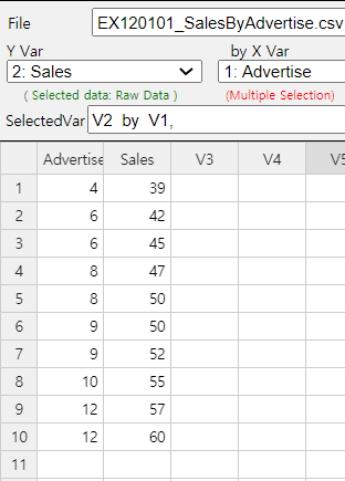
Using 『eStat』 , enter data as shown in <Figure 12.1.1>. If you select the Sales as 'Y Var' and the Advertise 'by X Var' in the variable selection box that appears when you click the scatter plot icon on the main menu, the scatter plot will appear as shown in <Figure 12.1.2>. As we can expect, the scatter plot show that the more investments in advertising, the more sales increase, and not only that, the form of increase is linear.
The same analysis of scatter plot can be done using 『eStatU』 by following data input and clicking [Execute] button..
[]
In order to understand the meaning of covariance, consider a case that \(Y\) increases if \(X\) increases. If the value of \(X\) is larger than \(\small \overline X\) and the value of \(Y\) is larger than \(\small \overline Y\), then \(\small (X - \overline X)(Y- \overline Y) \) always has a positive value. Also, if the value of \(X\) is smaller than \(\small \overline X\) and the value of \(Y\) is smaller than \(\small \overline Y\), then \(\small (X - \overline X)(Y- \overline Y) \) has a positive value. Therefore, their mean value which is the covariance tends to be positive. Conversely, if the value of the covariance is negative, the value of the other variable decreases as the value of one variable increases. Hence, by calculating covariance, we can see the relation between two variables: positive correlation (i.e., increasing the value of one variable will increase the value of the other) or negative correlation (i.e., decreasing the value of the other).
Covariance itself is a good measure, but, since the covariance depends on the unit of \(X\) and \(Y\), it makes difficult to interpret the covariance according to the size of the value and inconvenient to compare with other data. Standardized covariance which divides the covariance by the standard deviation of \(X\) and \(Y\), \(\sigma_{X}\) and \(\sigma_{Y}\), to obtain a measurement unrelated to the type of variable or specific unit, is called the population correlation coefficient and denoted as \(\rho\).
$$ \text{Population Correlation Coefficient: } \rho = \frac{Cov (X, Y)} { \sigma_X \sigma_Y } $$
<Figure 12.1.3> shows different scatter plots and its values of the correlation coefficient.
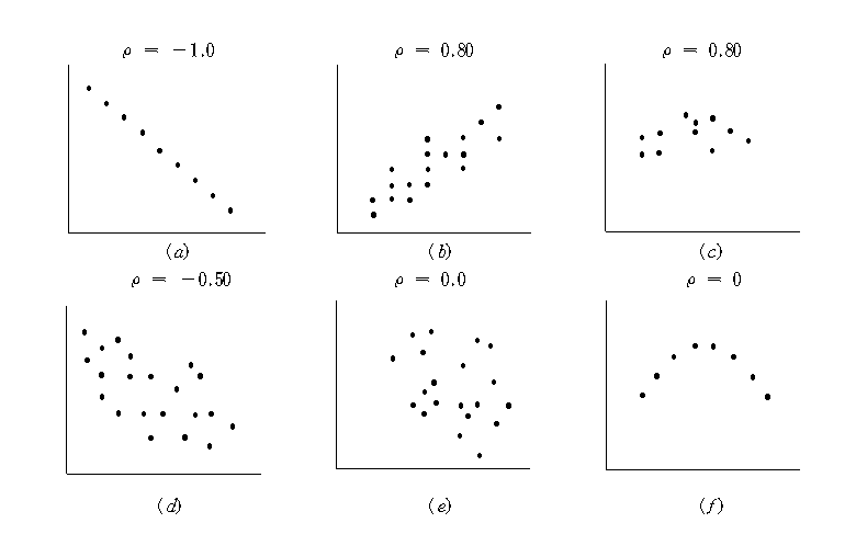
The correlation coefficient \(\rho\) is interpreted as follows:
『eStatU』 provides a simulation of scatter plot shapes for different correlations as in <Figure 12.1.4>.
[Correlation Simulation]
An estimate of the population correlation coefficient using samples of two variables is called the sample correlation coefficient and denoted as \(r\). The formula for the sample correlation coefficient \(r\) can be obtained by replacing each parameter with the estimates in the formula for the population correlation coefficient. $$ r = \frac {S_{XY}} { S_X S_Y } $$ where \(S_{XY}\) is the sample covariance and \(S_{X}\), \(S_{Y}\) are the sample standard deviations of \(X\) and \(Y\) as follows: $$\small \begin{align} S_{XY} &= \frac{1}{n-1} \sum_{i=1}^{n} (X_i - \overline X )(Y_i - \overline Y ) \\ S_X^2 &= \frac{1}{n-1} \sum_{i=1}^{n} (X_i - \overline X )^{2} \\ S_Y^2 &= \frac{1}{n-1} \sum_{i=1}^{n} (Y_i - \overline Y )^{2} \\ \end{align} $$ Therefore, the formula \(r\) can be written as follows $$\small \begin{align} r &= \frac {\sum_{i=1}^{n} (X_i - \overline X )(Y_i - \overline Y )} { \sqrt{\sum_{i=1}^{n} (X_i - \overline X )^{2} \sum_{i=1}^{n} (Y_i - \overline Y )^{2} } } \\ &= \frac {\sum_{i=1}^{n} X_i Y_i - n \overline X \overline Y } { \sqrt{\left (\sum_{i=1}^{n} X_{i}^{2} - n {\overline X}^2 \right) \left( \sum_{i=1}^{n} Y_{i}^{2} - n {\overline Y}^{2} \right) } } \end{align} $$
Example 12.1.2 Find the sample covariance and correlation coefficient for the advertising costs and sales of [Example 12.1.1].
Answer
To calculate the sample covariance and correlation coefficient, it is convenient to make the following table. This table can also be used for calculations in regression analysis.
| Number | \(X\) | \(Y\) | \(X^2\) | \(Y^2\) | \(XY\) |
|---|---|---|---|---|---|
| 1 | 4 | 39 | 16 | 1521 | 156 |
| 2 | 6 | 42 | 36 | 1764 | 252 |
| 3 | 6 | 45 | 36 | 2025 | 270 |
| 4 | 8 | 47 | 64 | 2209 | 376 |
| 5 | 8 | 50 | 64 | 2500 | 400 |
| 6 | 9 | 50 | 81 | 2500 | 450 |
| 7 | 9 | 52 | 81 | 2704 | 468 |
| 8 | 10 | 55 | 100 | 3025 | 550 |
| 9 | 12 | 57 | 144 | 3249 | 684 |
| 10 | 12 | 60 | 144 | 3600 | 720 |
| Sum | 64 | 497 | 766 | 25097 | 4326 |
| Mean | 8.4 | 49.7 |
Terms which are necessary to calculate the covariance and correlation coefficient are as follows:
\(\small \quad SXX = \sum_{i=1}^{n} (X_i - \overline X )^{2} = \sum_{i=1}^{n} X_{i}^2 - n{\overline X}^{2} = 766 - 10×8.4^2 = 60.4 \)
\(\small \quad SYY = \sum_{i=1}^{n} (Y_i - \overline Y )^{2} = \sum_{i=1}^{n} Y_{i}^2 - n{\overline Y}^{2} = 25097 - 10×49.7^2 = 396.1 \)
\(\small \quad SXY = \sum_{i=1}^{n} (X_i - \overline X )(Y_i - \overline Y ) = \sum_{i=1}^{n} X_{i}Y_{i} - n{\overline X}{\overline Y} = 4326 - 10×8.4×49.7 = 151.2 \)
\(\small SXX, SYY, SXY \)represent the sum of squares of \(\small X\), the sum of squares of \(\small Y\), the sum of squares of \(\small XY\). Hence, the covariance and correlation coefficient are as follows:
\(\small \quad S_{XY} = \frac{1}{n-1} \sum_{i=1}^{n} (X_i - \overline X )(Y_i - \overline Y ) = \frac{151.2}{10-1} = 16.8 \)
\(\small \quad r = \frac {\sum_{i=1}^{n} (X_i - \overline X )(Y_i - \overline Y )} { \sqrt{\sum_{i=1}^{n} (X_i - \overline X )^{2} \sum_{i=1}^{n} (Y_i - \overline Y )^{2} } } = \frac{151.2} { \sqrt{ 60.4 × 396.1 } } = 0.978 \)
This value of the correlation coefficient is consistent with the scatter plot which shows a strong positive correlation of the two variables.
Null Hypothesis: \(H_0 : \rho = 0\)
Test Statistic: \(\qquad t_0 = \sqrt{n-2} \frac{r}{\sqrt{1 - r^2 }}\), \( \quad t_0 \) follows \(t\) distribution with \(n-2\) degrees of freedom
Rejection Region of \(H_0\):
\( \qquad 1)\; H_1 : \rho < 0 , \;\;\) Reject if \(\; t_0 < -t_{n-2; α}\)
\( \qquad 2)\; H_1 : \rho > 0 , \;\;\) Reject if \(\; t_0 > t_{n-2; α}\)
\( \qquad 3)\; H_1 : \rho \ne 0 , \;\;\) Reject if \(\; |t_0 | > t_{n-2; α/2}\)
Example 12.1.3 In the Example 12.1.2, test the hypothesis that the population correlation coefficient between advertising cost and the sales amount is zero at the significance level of 0.05. (Since the sample correlation coefficient is 0.978 which is close to 1, this test will not be required in practice.)
Answer
The value of the test statistic \(t\) is as follows:
\(\qquad \small t_0 = \sqrt{10-2} \frac{0.978}{\sqrt{1 - 0.978^2 }}\) = 13.26
Since it is greater than \(t_{8; 0.025}\) = 2.306, \(\small H_0 : \rho = 0\) should be rejected.
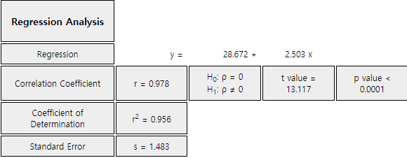
With the selected variables of 『eStat』 as <Figure 12.1.1>, click the regression icon on the main menu, then the scatter plot with a regression line will appear. Clicking the [Correlation and Regression] button below this graph will show the output as <Figure 12.1.5> in the Log Area with the result of the regression analysis. The values of this result are slightly different from the textbook, which is the error associated with the number of digits below the decimal point. The same conclusion is obtained that the p-value for the correlation test is 0.0001, less than the significance level of 0.05 and therefore, the null hypothesis is rejected.
| id | Mid-term X | Final Y |
|---|---|---|
| 1 | 92 | 87 |
| 2 | 65 | 71 |
| 3 | 75 | 75 |
| 4 | 83 | 84 |
| 5 | 95 | 93 |
| 6 | 87 | 82 |
| 7 | 96 | 98 |
| 8 | 53 | 42 |
| 9 | 77 | 82 |
| 10 | 68 | 60 |
Example 12.1.4 Draw a scatter plot matrix and correlation coefficient matrix using four variables of the iris data saved in the following location of 『eStat』.
The variables are Sepal.Length, Sepal.Width, Petal.Length, and Petal.Width. Test the hypothesis whether the correlation coefficients are equal to zero.
Answer
From 『eStat』, load the data and click the 'Regression' icon. When the variable selection box appears, select the four variables of Sepal.Length, Sepal.Width, Petal.Length, and Petal.Width, then the scatter plot matrix will be shown as <Figure 12.1.6>.
It is observed that the Sepal.Length and the Petal.Length, and the Petal.Length and the Petal.Width are related.
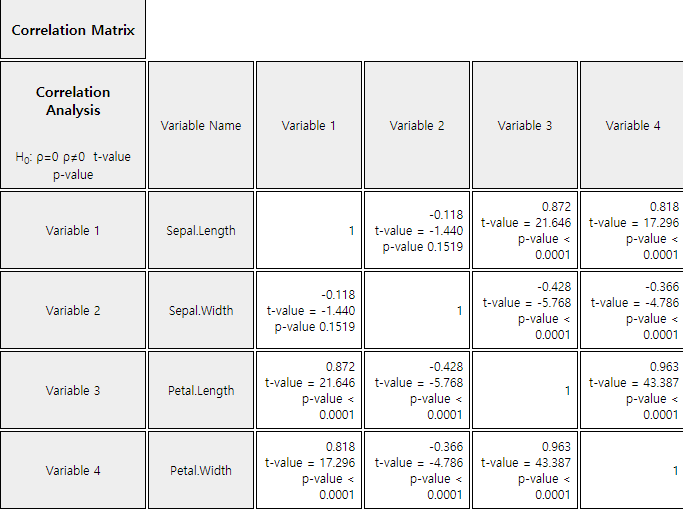
When selecting [Regression Analysis] button from the options below the graph, the basic statistics and correlation coefficient matrix such as <Figure 12.1.7> appear in the Log Area with the test result. It can be seen that all correlations are significant except the correlation coefficient between the Sepal.Length and Sepal.Width.

| smoking rate \(x_1\) |
ratio of weight by height \(x_2\) |
time to exercise \(y\) |
|---|---|---|
| 24 | 53 | 11 |
| 0 | 47 | 22 |
| 25 | 50 | 7 |
| 0 | 52 | 26 |
| 5 | 40 | 22 |
| 18 | 44 | 15 |
| 20 | 46 | 9 |
| 0 | 45 | 23 |
| 15 | 56 | 15 |
| 6 | 40 | 24 |
| 0 | 45 | 27 |
| 15 | 47 | 14 |
| 18 | 41 | 13 |
| 5 | 38 | 21 |
| 10 | 51 | 20 |
| 0 | 43 | 24 |
| 12 | 38 | 15 |
| 0 | 36 | 24 |
| 15 | 43 | 12 |
| 12 | 45 | 16 |
12.2 Simple Linear Regression Analysis
[presentation] [video]
Regression analysis is a statistical method that first establishes a reasonable mathematical model of relationships between variables, estimates the model using measured values of the variables, and then uses the estimated model to describe the relationship between the variables, or to apply it to the analysis such as forecasting.
If the number of independent variables included in the regression equation is one, it is called a simple linear regression. If the number of independent variables are two or more, it is called a multiple linear regression.
12.2.1 Simple Linear Regression Model
In order to estimate the regression coefficients \(\alpha\) and \(\beta\), observations of the dependent and independent variable are required, i.e., samples. In general, all of these observations are not located in a line. This is because, even if the \(Y\) and \(X\) have an exact linear relation, there may be a measurement error in the observations, or there may not be an exact linear relationship between \(Y\) and \(X\). Therefore, the regression formula can be written by considering these errors together as follows: $$ Y_i = \alpha + \beta X_i + \epsilon_{i}, \quad i=1,2,...,n $$ where \(i\) is the subscript representing the \(i^{th}\) observation, and \(\epsilon_i\) is the random variable indicating an error with a mean of zero and a variance \(\sigma^2\) which is independent of each other. The error \(\epsilon_i\) indicates that the observation \(Y_i\) is how far away from the population regression equation. The above equation includes unknown population parameters \(\alpha\), \(\beta\) and \(\sigma^2\), and is therefore, referred to as a population regression model.
If \(a\) and \(b\) are the estimated regression coefficients using samples, the fitted regression equation can be written as follows: It is referred to as the sample regression equation. $$ {\hat Y}_i = a + b X_i $$ In this expression, \({\hat Y}_i\) represents the estimated value of \(Y\) at \(X=X_i\) as predicted by the appropriate regression equation. These predicted values can not match the actual observed values of \(Y\), and differences between these two values are called residuals and denoted as \(e_i\). $$ \text{Residuals} \qquad e_i = Y_i - {\hat Y}_i , \quad i=1,2,...,n $$ The regression analysis makes some assumptions about the unobservable error \(\epsilon_i\). Since the residuals \(e_i\) calculated using the sample values have similar characteristics as \(\epsilon_i\), they are used to investigate the validity of these assumptions. (Refer to Section 12.2.6 for residual analysis.)
12.2.2 Estimation of Regression Coefficient
A method of estimating regression coefficients so that the total sum of the squared errors occurring in each observation is minimized. i.e.,
\(\quad\) Find \(\alpha\) and \(\beta\) which minimize
$$ \sum_{i=1}^{n} \epsilon_{i}^2 = \sum_{i=1}^{n} ( Y_i - \alpha - \beta X_i )^2 $$
The above expression is called a normal equation. The solution \(a\) and \(b\) of this normal equation is called the least squares estimator of \(\alpha\) and \(\beta\) and is given as follows:
\( \small \quad b = \frac {\sum_{i=1}^{n} (X_i - \overline X ) (Y_i - \overline Y )} { \sum_{i=1}^{n} (X_i - \overline X )^2 } \)
\( \small \quad a = \overline Y - b \overline X \)
Example 12.2.1 In [Example 12.1.1], find the least squares estimate of the slope and intercept if the sales amount is a dependent variable and the advertising cost is an independent variable. Predict the amount of sales when you have spent on advertising by 10.
Answer
In [Example 12.1.1], the calculation required to obtain the intercept and slope has already been made. The intercept and slope using this are as follows:
\( \quad b = \small \frac {\sum_{i=1}^{n} (X_i - \overline X ) (Y_i - \overline Y )} { \sum_{i=1}^{n} (X_i - \overline X )^2 } \\ = \frac {151.2}{60.4} = 2.503 \) \( \quad a = \small \overline Y - b \overline X = 49.7 - 2.503 \times 8.4 = 28.672 \)
Therefore, the fitted regression line is \(\small \hat Y_i = 28.672 + 2.503 X_i \).
<Figure 12.2.1> shows the fitted regression line on the original data. The meaning of slope value, 2.5033, is that, if advertising cost increases by one (i.e., one million), sales increases by about 2.5 million.
Prediction of the sales amount of a company with an advertising cost of 10 can be obtained by using the fitted sample regression line as follows:
\(\quad \small 28.672 + (2.503)(10) = 53.702 \)
In other words, sales of 53.705 million are expected. That is not to say that all companies with advertising costs of 10 million USD have sales of 53.705 million USD, but that the average amount of their sales is about that. Therefore, there may be some differences in individual companies.
The same analysis of scatter plot can be done using 『eStatU』 by following data input and clicking [Execute] button..
[]
12.2.3 Goodness of Fit for Regression Line
Residual standard error \(s\) is a measure of the extent to which observations are scattered around the estimated line. First, you can define the sample variance of residuals as follows: $$ s^2 = \frac{1}{n-2} \sum_{i=1}^{n} ( Y_i - {\hat Y}_i )^2 $$ The residual standard error \(s\) is defined as the square root of \(s^2\). The \(s^2\) is an estimate of \(\sigma^2\) which is the extent that the observations \(Y\) are spread around the population regression line. A small value of \(s\) or \(s^2\) indicates that the observations are close to the estimated regression line, which in turn implies that the regression line represents well the relationship between the two variables.
However, it is not clear how small the residual standard error \(s\) is, although the smaller value is the better. In addition, the size of the value of \(s\) depends on the unit of \(Y\). To eliminate this shortcoming, a relative measure called the coefficient of determination is defined. The coefficient of determination is the ratio of the variation described by the regression line over the total variation of observation \(Y_i\), so that it is a relative measure that can be used regardless of the type and unit of the variable.
As in the analysis of variance in Chapter 9, the following partitions of the sum of squares and degrees of freedom are formed in the regression analysis:
\(\qquad\) Sum of squares: \(\qquad SST = SSE + SSR\)
\(\qquad\) Degrees of freedom: \((n-1) = (n-2) + 1\)
Total Sum of Squares : \( \small SST = \sum_{i=1}^{n} ( Y_i - {\overline Y} )^2\)
The total sum of squares indicating the total variation in observed values of \(Y\) is called the total sum of squares (\(SST\)). This \(SST\) has the degree of freedom, \(n-1\), and if \(SST\) is divided by the the degree of freedom, it becomes the sample variance of \(Y_i\).
Error Sum of Squares : \( \small SSE = \sum_{i=1}^{n} ( Y_i - {\hat Y}_i )^2\)
The error sum of squares (\(SSE\)) of the residuals represents the unexplained variation of the total variation of the \(Y\). Since the calculation of this sum of squares requires the estimation of two parameters \(\alpha\) and \(\beta\), \(SSE\) has the degree of freedom \(n-2\). This is the reason why, in the calculation of the sample variance of residuals \(s^2\), it was divided by \(n-2\).
Regression Sum of Squares : \( \small SSR = \sum_{i=1}^{n} ( {\hat Y}_i - {\overline Y} )^2 \)
The regression sum of squares (\(SSR\)) indicates the variation explained by the regression line among the total variation of \(Y\). This sum of squares has the degree of freedom of 1.
If the estimated regression equation fully explains the variation in all samples (i.e., if all observations are on the sample regression line), the unexplained variation \(SSE\) will be zero. Thus, if the portion of \(SSE\) is small among the total sum of squares \(SST\), or if the portion of \(SSR\) is large, the estimated regression model is more suitable. Therefore, the ratio of \(SSR\) to the total variation \(SST\), called the coefficient of determination, is defined as a measure of the suitability of the regression line as follows: $$ R^2 = \frac{Explained \;\; Variation}{Total \;\; Variation} = \frac{SSR}{SST} $$ The value of the coefficient of determination is always between 0 and 1 and the closer the value is to 1, the more concentrated the samples are around the regression line, which means that the estimated regression line explains the observations well.
Example 12.2.2 Calculate the value of the residual standard error and the coefficient of determination in the data on advertising costs and sales.
Answer
To obtain the residual standard error and the coefficient of determination, it is convenient to make the following Table 12.2.1. Here, the estimated value \(\small {\hat Y}_i\) of the sales from each value of \(\small {X}_i\) uses the fitted regression line.
\( \qquad \small {\hat Y}_i = 28.672 + 2.503 X_i \)
| Number | \(\small X_i\) | \(\small Y_i\) | \(\small {\hat Y}_i\) | \(\small SST\) \(\small (Y_i - {\overline Y}_i )^2 \) |
\(\small SSR\) \(\small ({\hat Y}_i - {\overline Y}_i )^2 \) |
\(\small SSE\) \(\small (Y_i - {\hat Y}_i )^2 \) |
|---|---|---|---|---|---|---|
| 1 | 4 | 39 | 38.639 | 114.49 | 122.346 | 0.130 |
| 2 | 6 | 42 | 43.645 | 59.29 | 36.663 | 2.706 |
| 3 | 6 | 45 | 43.645 | 22.09 | 36.663 | 1.836 |
| 4 | 8 | 47 | 48.651 | 7.29 | 1.100 | 2.726 |
| 5 | 8 | 50 | 48.651 | 0.09 | 1.100 | 1.820 |
| 6 | 9 | 50 | 51.154 | 0.09 | 2.114 | 1.332 |
| 7 | 9 | 52 | 51.154 | 5.29 | 2.114 | 0.716 |
| 8 | 10 | 55 | 53.657 | 28.09 | 15.658 | 1.804 |
| 9 | 12 | 57 | 58.663 | 53.29 | 80.335 | 2.766 |
| 10 | 12 | 60 | 58.663 | 106.09 | 80.335 | 1.788 |
| Sum | 64 | 497 | 496.522 | 396.1 | 378.429 | 17.622 |
| Average | 8.4 | 49.7 |
In Table 12.2.1, \(\small SST\) = 396.1, \(\small SSR\) = 378.429, \(\small SSE\) = 17.622. Here, the relationship of \(\small SST = SSE + SSR\) does not exactly match because of the error in the number of digits calculation. The sample variance of residuals is as follows:
\(\qquad \small s^2 = \frac{1}{n-2} \sum_{i=1}^{n} ( Y_i - {\hat Y}_i )^2 = \frac{17.622}{(10-2)} = 2.203 \)
Hence, the residual standard error is \(s\) = 1.484. The coefficient of determination is as follows:
\(\qquad \small R^2 = \frac{SSR}{SST} = \frac{378.429}{396.1} = 0.956\)
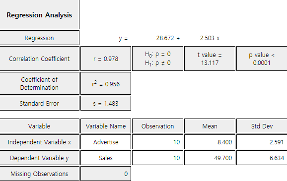
This means that 95.6% of the total variation in the observed 10 sales amounts can be explained by the simple linear regression model using a variable of advertising costs, so this regression line is quite useful.
Click the [Correlation and Regression] button in the option below the graph of <Figure 12.2.1> to show the coefficient of determinations and estimation errors shown in <Figure 12.2.2>.
12.2.4 Analysis of Variance for Regression
| Source | Sum of squares | Degrees of freedom | Mean Squares | F value |
|---|---|---|---|---|
| Regression | SSR | 1 | MSR =\(\frac{SSR}{1}\) | \(F_0 = \frac{MSR}{MSE}\) |
| Error | SSE | \(n-2\) | MSE = \(\frac{SSE}{n-2}\) | |
| Total | SST | \(n-1\) |
The \(F\) value given in the last column are used for testing hypothesis \(H_0: \beta = 0 ,\; H_1 : \beta \ne 0 \). If \(\beta\) is not 0, the \(F\) value can be expected to be large, because the assumed regression line is valid and the variation of \(Y\) is explained in large part by the regression line. Therefore, we can reversely decide that \(\beta\) is not zero if the calculated \(F\) ratio is large enough. If the assumptions about the error terms mentioned in the population regression model are valid and if the error terms follows a normal distribution, the distribution of \(F\) value, when the null hypothesis is true, follows \(F\) distribution with 1 and \(n-2\) degrees of freedom. Therefore, if \(F_0 > F_{1,n-2; α}\), then we can reject \(H_0 : \beta = 0\) .
\(\quad \) Hypothesis: \(H_0 : \beta = 0, \;\; H_1 : \beta \ne 0\)
\(\quad \) Decision rule: If \({F_0} = \frac{MSR}{MSE} > F_{1, n-2; α}\), then reject \(H_0\)
(In 『eStat』, the \(p\)-value for this test is calculated and the decision can be made using this \(p\)-value. That is, if the \(p\)-value is less than the significance level, the null hypothesis \(H_0\) is rejected.)
Example 12.2.3 Prepare an ANOVA table for the example of advertising cost and test it using the 5% significance level.
Answer
Using the sum of squares calculated in [Example 12.2.2], the ANOVA table is prepared as follows:
| Source | Sum of squares | Degrees of freedom | Mean Squares | \(\small F\) value |
|---|---|---|---|---|
| Regression | 378.42 | 1 | MSR = \(\frac{378.42}{1}\) = 378.42 | \(F_0 = \frac{378.42}{2.20}\) |
| Error | 17.62 | 10-2 | MSE = \(\frac{17.62}{8} = 2.20\) | |
| Total | 396.04 | 10-1 |
Since the calculated \(\small F\) value of 172.0 is much greater than \(\small F_{1,8; 0.05} = 5.32 \), we reject the null hypothesis \(\small H_0 : \beta = 0\) with the significance level \(\alpha\) = 0.05.
Click the [Correlation and Regression] button in the options window below the graph <Figure 12.2.1> to show the result of the ANOVA as shown in <Figure 12.2.3>.

12.2.5 Inference for Regression
Point estimate: \(\small \quad b = \frac {\sum_{i=1}^{n} (X_i - \overline X) (Y_i - \overline Y)} { \sum_{i=1}^{n} (X_i - \overline X)^2 } , \quad b \sim N(\beta, \frac{\sigma^2} {\sum_{i=1}^{n} (X_i - \overline X )^2 } ) \)
Standard error of estimate \(b\): \(\small \quad SE(b) = \frac{s}{\sqrt {{\sum_{i=1}^{n} (X_i - \overline X)^2} } }\)
Confidence interval of \(\; \beta\): \(\quad b \pm t_{n-2; α/2} \cdot SE(b)\)
Testing hypothesis:
\(\quad\) Null hypothesis: \(\quad H_0 : \beta = \beta_0\)
\(\quad\) Test statistic: \(\quad t = \frac{b - \beta_0 } { SE (b) }\)
\(\quad\) rejection region:
\(\qquad\) if \(H_1 : \beta \lt \beta_0\), then \(\; t < - t_{n-2; α}\)
\(\qquad\) if \(H_1 : \beta \gt \beta_0\), then \(\; t > t_{n-2; α}\)
\(\qquad\) if \(H_1 : \beta \ne \beta_0\), then \(\; |t| > t_{n-2; α/2}\)
Point estimate: \(\quad \small a = \overline Y - b \overline X , \quad a \sim N( \alpha, ( \frac{1}{n} + \frac {{\overline X }^2} { \sum_{i=1}^{n} (X_i - \overline X )^2 } ) \cdot \sigma^2 ) \)
Standard error of estimate \(a\): \(\small \quad SE(a) = s \cdot \sqrt {\frac{1}{n} + \frac {{\overline X }^2} { \sum_{i=1}^{n} (X_i - \overline X )^2 } ) } \)
Confidence interval of \(\; \alpha\): \(\quad a \pm t_{n-2; α/2} \cdot SE(a)\)
Testing hypothesis:
\(\quad\) Null hypothesis: \(\quad H_0 : \alpha = \alpha_0\)
\(\quad\) Test statistic: \(\quad t = \frac{a - \alpha_0 } { SE (a) }\)
\(\quad\) rejection region:
\(\qquad\) if \(H_1 : \alpha \lt \alpha_0\), then \(\; t < - t_{n-2; α}\)
\(\qquad\) if \(H_1 : \alpha \gt \alpha_0\), then \(\; t > t_{n-2; α}\)
\(\qquad\) if \(H_1 : \alpha \ne \alpha_0\), then \(\; |t| > t_{n-2; α/2}\)
Point estimate: \(\quad {\hat Y}_0 = a + b X_0 \)
Standard error of estimate \({\hat Y}_0\): \(\small \quad SE({\hat Y}_0) = s \cdot \sqrt { \frac{1}{n} + \frac { (X_0 - \overline X )^2} { \sum_{i=1}^{n} (X_i - \overline X )^2 } } \)
Confidence interval of \(\; \mu_{Y|x}\): \(\quad {\hat Y}_0 \pm t_{n-2; α/2} \cdot SE ({\hat Y}_0 )\)
Example 12.2.4 Let's make inferences about each parameter with the result of a regression analysis of the previous data for the sales amount and advertising costs. Use 『eStat』 to check the test result and confidence band.
Answer
\(\quad \small SE(b) = \frac{s}{\sqrt {{\sum_{i=1}^{n} (X_i - \overline X)^2} } } = \frac{1.484}{\sqrt 60.4} = 0.1908\)
Hence, the 95% confidence interval of \(\beta\) using \(t_{8; 0.025} \) = 2.056 is as follows:
\(\quad \small 2.5033 \pm (2.056)(0.1908)\)
\(\quad \small 2.5033 \pm 0.3922\)
\(\quad\) i.e. the interval (2.1110, 2.8956).
The test statistic for the hypothesis \(\small H_0 : \beta = 0\), is as follows:
\(\quad t= \frac{2.5033 - 0}{0.1908}\) = 13.12
Since \(t_{8; 0.025} \) = 2.056, the null hypothesis \(\small H_0 : \beta = 0\) is rejected with the significance level of \(\alpha\) = 0.05. This result of two sided test can be obtained from the confidence interval. Since 95% confidence interval (1.7720, 3.2346) do not include 0, the null hypothesis \(\small H_0 : \beta = 0\) can be rejected.
\(\quad \small SE(a) = s \cdot \sqrt {\frac{1}{n} + \frac {{\overline X }^2} { \sum_{i=1}^{n} (X_i - \overline X )^2 } } = 1.484 \cdot \sqrt { \frac{1}{10} + \frac{8.4^2}{60.4} } \) = 1.670
Since the value of \(t\) statistic is \(\frac{29.672}{1.67}\) = 17.1657 and \(t_{8; 0.025}\) = 2.056, the null hypothesis \(\small H_0 : \alpha = 0\) is also rejected with the significance level \(\alpha\) = 0.05.
\(\small \quad SE({\hat Y}_0) = s \cdot \sqrt { \frac{1}{n} + \frac { (X_0 - \overline X )^2} { \sum_{i=1}^{n} (X_i - \overline X )^2 } } \)
\(\small \qquad \qquad \; = 1.484 \cdot \sqrt { \frac{1}{10} + \frac { (8 - 8.4)^2} {60.4 } }= 0.475 \)
Hence, the 95% confidence interval of \(\mu_{Y|x}\) is as follows:
\(\quad \small 48.696 \pm (2.056)×(0.475)\)
\(\quad \small 48.696 \pm 0.978\)
\(\quad\) i.e., the inteval is (47.718, 49.674).
We can calculate the confidence interval for other value of \(\small X\) in a similar way as follows:
\(\quad \) At \(\small \;X = 4, \quad 38.684 \pm (2.056)×(0.962) \Rightarrow (36.705, 40.663)\)
\(\quad \) At \(\small \;X = 6, \quad 47.690 \pm (2.056)×(0.656) \Rightarrow (42.341, 45.039)\)
\(\quad \) At \(\small \;X = 9, \quad 51.199 \pm (2.056)×(0.483) \Rightarrow (50.206, 52.192)\)
\(\quad \) At \(\small \;X =12, \quad 58.708 \pm (2.056)×(0.832) \Rightarrow (56.997, 60.419)\)
As we discussed, the confidence interval becomes wider as \(\small X\) is far from \(\small \overline X\).
If you select the [Confidence Band] button from the options below the regression graph of <Figure 12.2.1>, you can see the confidence band graph on the scatter plot together with regression line as <Figure 12.2.4>. If you click the [Correlation and Regression] button, the inference result of each parameter will appear in the Log Area as shown in <Figure 12.2.5>.

12.2.6 Residual Analysis
First, let's look at the assumptions in the regression model.
Assumptions in regression model
\(\quad \;\; A_1\): The assumed model \(Y = \alpha + \beta X + \epsilon\) is correct.
\(\quad \;\; A_2\): The expectation of error terms \(\epsilon_i\) is 0.
\(\quad \;\; A_3\): (Homoscedasticity) The variance of \(\epsilon_i\) is \(\sigma^2\) which is the same for all \(X\).
\(\quad \;\; A_4\): (Independence) Error terms \(\epsilon_i\) are independent.
\(\quad \;\; A_5\): (Normality) Error terms \(\epsilon_i\)’s are normally distributed.
Review the references for the meaning of these assumptions. The validity of these assumptions is generally
investigated using scatter plots of the residuals. The following scatter plots used primarily for each
assumption:
\(\quad \)1) Residuals versus predicted values (i.e., \(e_i\) vs \(\hat Y_i\)) : \(\quad A_3\)
\(\quad \)2) Residuals versus independent variables (i.e., \(e_i\) vs \(X_i\)) : \(\quad A_1\)
\(\quad \)3) Residuals versus observations (i.e., \(e_i\) vs \(i\)) : \(\quad A_2 , A4\)
In the above scatter plots, if the residuals show no particular trend around zero, and appear randomly,
then each assumption is valid.
The assumption that the error term \(\epsilon\) follows a normal distribution can be investigated
by drawing a histogram of the residuals in case of a large amount of data to see if the distribution
is similar to the shape of the normal distribution. Another method is to use the quantile–quantile (Q-Q)
scatter plot of the residuals. In general, if the Q-Q scatter plot of the residuals forms a straight line,
it can be considered as a normal distribution.
Since residuals are also dependent on the unit of the dependent variable, standardized values of
the residuals are used for consistent analysis of the residuals, which are called standardized residuals.
Both the scatter plots of the residuals described above and the Q-Q scatter plot are created using
the standardized residuals. In particular, if the value of the standardized residuals is outside
the \(\pm\)2, an anomaly value or an outlier value can be suspected.
Example 12.2.5 Draw a scatter plot of residuals and a Q-Q scatter plot for the advertising cost example.
Answer
When you click the [Residual Plot] button from the options below the regression graph of <Figure 12.2.1>, the scatter plot of the standardized residuals and predicted values are appeared as shown in <Figure 12.2.6>. If you click [Residual Q-Q Plot] button, <Figure 12.2.7> is appeared. Although the scatter plot of the residuals has no significant pattern, the Q-Q plot deviates much from the straight line and so, the normality of the error term is somewhat questionable. In such cases, the values of the response variable need to be re-analyzed by taking logarithmic or square root transformation.
[Regression Experiment ]
12.3 Multiple Linear Regression Analysis
[presentation] [video]
12.3.1 Multiple Linear Regression Model
Example 12.3.1 When logging trees in forest areas, it is necessary to investigate the amount of timber in those areas. Since it is difficult to measure the volume of a tree directly, we can think of ways to estimate the volume using the diameter and height of a tree that is relatively easy to measure. The data in Table 12.3.1 are the values for measuring diameter, height and volume after sampling of 15 trees in a region. (The diameter was measured at a point 1.5 meters above the ground.) Draw a scatter plot matrix of this data and consider a regression model for this problem.
| Diameter(\(cm\)) | Height(\(m\)) | Volume(\(m^3\)) |
|---|---|---|
| 21.0 | 21.33 | 0.291 |
| 21.8 | 19.81 | 0.291 |
| 22.3 | 19.20 | 0.288 |
| 26.6 | 21.94 | 0.464 |
| 27.1 | 24.68 | 0.532 |
| 27.4 | 25.29 | 0.557 |
| 27.9 | 20.11 | 0.441 |
| 27.9 | 22.86 | 0.515 |
| 29.7 | 21.03 | 0.603 |
| 32.7 | 22.55 | 0.628 |
| 32.7 | 25.90 | 0.956 |
| 33.7 | 26.21 | 0.775 |
| 34.7 | 21.64 | 0.727 |
| 35.0 | 19.50 | 0.704 |
| 40.6 | 21.94 | 1.084 |
Answer
Load the data saved at the following location of 『eStat』.
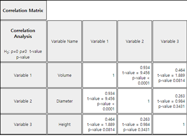
In the variable selection box which appears by selecting the regression icon, select 'Y variable' by volume and select ‘by X variable’ as the diameter and height to display a scatter plot matrix as shown in <Figure 12.3.1>. It can be observed that there is a high correlation between volume and diameter, and that volume and height, and diameter and height are also somewhat related.
Since the volume is to be estimated using the diameter and height of the tree, the volume is the dependent variable \(\small Y\), and the diameter and height are independent variables \(\small X_1 , X_2\) respectively, and the following regression model can be considered.
\(\quad Y_i = \beta_0 + \beta_1 X_{i1} + \beta_2 X_{i2} + \epsilon_i , \quad i=1,2,...,15\)
The same analysis of multiple linear regression can be done using 『eStatU』 by following data input and clicking [Execute] button..
[]
| smoking rate \(x_1\) |
ratio of weight by height \(x_2\) |
time to continue to exercise \(y\) |
|---|---|---|
| 24 | 53 | 11 |
| 0 | 47 | 22 |
| 25 | 50 | 7 |
| 0 | 52 | 26 |
| 5 | 40 | 22 |
| 18 | 44 | 15 |
| 20 | 46 | 9 |
| 0 | 45 | 23 |
| 15 | 56 | 15 |
| 6 | 40 | 24 |
| 0 | 45 | 27 |
| 15 | 47 | 14 |
| 18 | 41 | 13 |
| 5 | 38 | 21 |
| 10 | 51 | 20 |
| 0 | 43 | 24 |
| 12 | 38 | 15 |
| 0 | 36 | 24 |
| 15 | 43 | 12 |
| 12 | 45 | 16 |
Here \(\mathbf {Y, X}, \boldsymbol{\beta , \epsilon}\) are defined as follows: $$ {\bf Y} = \left[ \matrix{ Y_1 \\ Y_2 \\ \cdot \\ \cdot \\ Y_n } \right], \quad {\bf X} = \left[ \matrix{ 1 & X_{11} & X_{12} & \cdots & X_{1k} \\ 1 & X_{21} & X_{22} & \cdots & X_{2k} \\ & & \cdots \\ & & \cdots \\ 1 & X_{n1} & X_{n2} & \cdots & X_{nk} } \right], \quad {\boldsymbol \beta} = \left[ \matrix{ \beta_0 \\ \beta_1 \\ \cdot \\ \cdot \\ \beta_k } \right], \quad {\boldsymbol \epsilon} = \left[ \matrix{ \epsilon_1 \\ \epsilon_2 \\ \cdot \\ \cdot \\ \epsilon_n } \right] $$
12.3.2 Estimation of Regression Coefficient
If the estimated regression coefficients are \({\bf b} = (b_0 , b_1 , ... , b_k )\), the estimate of the response variable \(Y\) is as follows: $$ {\hat Y}_i = b_0 + b_1 X_{i1} + \cdots + b_k X_{ik} $$ The residuals are as follows: $$ \begin{align} e_i &= Y_i - {\hat Y}_i \\ &= Y_i - (b_0 + b_1 X_{i1} + \cdots + b_k X_{ik} ) \end{align} $$ By using a vector notation, the residual vector \(\bf e\) can be defined as follows: $$ \bf {e = Y - X b} $$
12.3.3 Goodness of Fit for Regression and Analysis of Variance
In the multiple linear regression analysis, the standard error of residuals is defined as follows: $$ s = \sqrt { \frac{1}{n-k-1} \sum_{i=1}^{n} (Y_i - {\hat Y}_i )^2} $$ The difference from the simple linear regression is that the degrees of freedom for residuals is \(n-k-1\), because the \(k\) number of regression coefficients must be estimated in order to calculate residuals. As in simple linear regression, \(s^2\) is a statistic such as the residual mean squares (\(MSE\)). The coefficient of determination is given in \(R^2 = \frac{SSR}{SST}\) and its interpretation is as shown in the simple linear regression.
The sum of squares is defined by the same formula as in the simple linear regression, and can be divided with
corresponding degrees of freedom as follows and the table of the analysis of variance is shown in Table 12.3.2.
\(\quad\) Sum of squares \(\quad \quad \;\;SST = SSE + SSR\)
\(\quad\) Degrees of freedom \(\quad (n-1) = (n-k-1) + k\)
| Source | Sum of squares | Degrees of freedom | Mean Squares | F value |
|---|---|---|---|---|
| Regression | SSR | \(k\) | MSR = \(\frac{SSR}{k}\) | \(F_0 = \frac{MSR}{MSE}\) |
| Error | SSE | \(n-k-1\) | MSE = \(\frac{SSE}{n-k-1}\) | |
| Total | SST | \(n-1\) |
12.3.4 Inference for Multiple Linear Regression
Point estimate: \(\quad b_i \)
Standard error of estimate \(b\): \(\quad SE(b_i) = \sqrt c_{ii} \cdot s \)
Confidence interval of \(\; \beta_i\): \(\quad b_i \pm t_{n-k-1; α/2} \cdot SE(b_i)\)
Testing hypothesis:
\(\quad\) Null hypothesis: \(\quad H_0 : \beta_i = \beta_{i0}\)
\(\quad\) Test statistic: \(\quad t = \frac{b_i - \beta_{i0} } { SE (b_i) }\)
\(\quad\) rejection region:
\(\qquad\) if \(\; H_1 : \beta_i \lt \beta_{i0}\), then \(\; t < - t_{n-k-1; α}\)
\(\qquad\) if \(\; H_1 : \beta_i \gt \beta_{i0}\), then \(\; t > t_{n-k-1; α}\)
\(\qquad\) if \(\; H_1 : \beta_i \ne \beta_{i0}\), then \(\; |t| > t_{n-k-1; α/2}\)
(Since 『eStat』 calculates the \(p\)-value under the null hypothesis \(H_0 : \beta_i = \beta_{i0}\),
\(p\)-value is used for testing hypothesis. )
Example 12.3.2 For the tree data of [Example 12.3.1], obtain the least squares estimate of each coefficient of the proposed regression equation using 『eStat』 and apply the analysis of variance, test for goodness of fit and test for regression coefficients.
Answer
In the options window below the scatter plot matrix in <Figure 12.3.1>, click [Regression Analysis] button. Then you can find the estimated regression line, ANOVA table as shown in <Figure 12.3.3> in the Log Area. The estimated regression equation is as follows:
\(\quad \small {\hat Y}_i = -1.024 + 0.037 X_1 + 0.024 X_2 \)
In the above equation, 0.037 represents the increase of the volume of the tree when the diameter (\(\small X_1\)) increases 1(cm).
The \(p\)-value calculated from the ANOVA table in <Figure 12.3.3> at \(\small F\) value of 73.12 is less than 0.0001, so you can reject the null hypothesis \(\small H_0 : \beta_1 = \beta_{2} = 0\) at the significance level \(\alpha\) = 0.05. The coefficient of determination, \(\small R^2\) = 0.924, implies that 92.4% of the total variances of the dependent variable are explained by the regression line. Based on the above two results, we can conclude that the diameter and height of the tree are quite useful in estimating the volume.
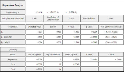
Since \(\small {SE}(b_1 ) = 0.003, \; {SE} (b_2 ) = 0.008 \) and \(t_{12; 0.025}\) = 2.179 from the result in <Figure 12.3.3>, the 95% confidence intervals for each regression coefficients can be calculated as follows: The difference between this result and the <Figure 12.3.3> due to the error in the calculation below the decimal point.
\(\quad \) 95% confidence interval for \(\beta_1 : \;\; \) 0.037 \(\pm\) (2.179)(0.003) \(\Rightarrow\) (0.029, ~0.045)
\(\quad \) 95% confidence interval for \(\beta_2 : \;\; \) 0.024 \(\pm\) (2.179)(0.008) \(\Rightarrow\) (0.006,~ 0.042)
In the hypothesis test of \(\small H_0 : \beta_i = 0 , \;\; H_1 : \beta_i \ne 0\) , each \(p\)-value is less than the significance level of 0.05, so you can reject each null hypothesis.
The scatter plot of the standardized residuals is shown in <Figure 12.3.4> and the Q-Q scatter plot is shown in <Figure 12.3.5>. There is no particular pattern in the scatter plot of the standardized residuals, but there is one outlier value, and the Q-Q scatter plot shows that the assumption of normality is somewhat satisfactory.