Chapter 11. Testing Hypothesis for Categorical Data
[book] [eStat YouTube Channel]
CHAPTER OBJECTIVES
The hypothesis tests that we have studied from Chapter 7 to Chapter 10 are for continuous data. In this chapter, we describe testing hypothesis for categorical data. Section 11.1 describes the goodness of fit test for the frequency table of categorical data. Section 11.2 describes the independence and homogeneity tests for the contingence table of two categorical data.
11.1 Goodness of Fit Test
[presentation] [video]
11.1.1 Goodness of Fit Test for Categorical Distribution
Example 11.1.1 The result of a survey of 150 people before a local election to find out the approval ratings of three candidates is as follows. Looking at this frequency table alone, it seems that A candidate has a 40 percent approval rating, higher than the other candidates. Based on this sample survey, perform the goodness of fit test whether three candidates have the same approval rating or not. Use 『eStatU』 with the 5% significance level.
| Candidate | Number of Supporters | Percent |
|---|---|---|
| A | 60 | 40.0% |
| B | 50 | 33.3% |
| C | 40 | 25.7% |
| Total | 150 | 100.0% |
Answer
Assume each of candidate A, B, and C’s approval rating is \(p_1 , p_2 , p_3\) respectively. The hypothesis for this problem is as follows:
If the null hypothesis \(\small H_0\) is true that the three candidates have the same approval rating, each candidate will have 50 (= 150\(\times \frac{1}{3}\) ) supporters out of total 150 people. It is referred to as the ‘expected frequency’ of each candidate when \(\small H_0\) is true. For each candidate, the number of observed supporters in the sample is called the 'observed frequency'. If \(\small H_0\) is true, the observed and expected number of supporters can be summarized as the following table.
| Candidate | Observed frequency (denoted as \(O_i\)) |
Expected frequency (denoted as \(E_i\)) |
|---|---|---|
| A | \(O_1 = 60\) | \(E_1 = 50\) |
| B | \(O_2 = 50\) | \(E_2 = 50\) |
| C | \(O_3 = 40\) | \(E_3 = 50\) |
| Total | 150 | 150 |
If \(\small H_0\) is true, the observed frequency (\(\small O_i\)) and the expected frequency (\(\small E_i\)) will coincide. Therefore, in order to test the hypothesis, a statistic which uses the squared difference between \(\small O_i\) and \(\small E_i\) is used. Specifically, the statistic to test the hypotheses is as follows:
If the observed value of this test statistic is close to zero, it can be considered that \(\small H_0\) is true, because \(\small O_i\) is close to \(\small E_i\). If the observed value is large, \(\small H_0\) will be rejected. The question is, 'How large value of the test statistic would be considered as the statistically significant one?' It can be shown that this test statistic approximately follows the chi-square distribution with \(k-1\) degrees of freedom if the expected frequency is large enough. Here \(k\) is the number of categories (i.e., candidates) in the table and it is 3 in this example. Therefore, the decision rule to test the hypotheses is as follows:
The statistic \(\chi_{obs}^2\) can be calculated as follows:
Since the significance level α is 5%, the critical value can be found from the chi-square distribution as follows:
Therefore, \(\small H_0\) cannot be rejected. In other words, although the above sample frequency table shows that the approval ratings of the three candidates differ, this difference does not provide sufficient evidence to conclude that the three candidates have different approval ratings.
Since sample approval ratings of each candidate are \(\hat p_1 = \frac{60}{150}\) = 0.40, \(\hat p_2 = \frac{50}{150}\) = 0.33, \(\hat p_3 = \frac{40}{150}\) = 0.27, the 95% confidence intervals for the population proportion of each candidate's approval rating using the formula (\( {{\hat p}} ± 1.96 \sqrt { \hat p (1- \hat p ) / n } \)) (refer Chapter 6.4) are as follows:
B: \( \quad 0.33 \pm 1.96 \sqrt { \frac {0.33 \times 0.67} {150} } \quad \quad \Leftrightarrow \quad \) [0.255, 0.405]
C: \( \quad 0.27 \pm 1.96 \sqrt { \frac {0.27 \times 0.73} {150} } \quad \quad \Leftrightarrow \quad \) [0.190, 0.330]
The overlapping of the confidence intervals on the three candidates' approval ratings means that one candidate's approval rating is not completely different from the other.
In the data input box that appears by selecting the [Goodness of Fit Test] of 『eStatU』, enter the 'Observed Frequency' and 'Expected Probability' data as shown in <Figure 11.1.1>. After entering the data, select the significance level and click [Execute] button to calculate the 'Expected Frequency' and to see the result of the chi-square test. Be sure that this chi-square goodness of fit test should be applied when the expected frequency of each category is at least 5.
[]
| \(X\) | \(P(X = x)\) |
|---|---|
| \(x_1\) | \(p_1\) |
| \(x_2\) | \(p_2\) |
| \(\cdots\) | \(\cdots\) |
| \(x_k\) | \(p_k\) |
| Total | 1 |
When random samples are collected from the population of the categorical random variable X and their
observed frequencies are (\(O_1 , O_2 , ... , O_k \)), the hypothesis to test the population probability
distribution of (\(p_1 , p_2 , ... , p_k \)) = (\(p_{10} , p_{20} , ... , p_{k0} \)) is as follows:
\(\qquad H_0\) : Distribution of (\(O_1 , O_2 , ... , O_k \)) are from the distribution (\(p_1 , p_2 , ... , p_k \)) = (\(p_{10} , p_{20} , ... , p_{k0} ) \)
\(\qquad H_1\) : Distribution of (\(O_1 , O_2 , ... , O_k \)) are not from the distribution (\(p_1 , p_2 , ... , p_k \)) = (\(p_{10} , p_{20} , ... , p_{k0} ) \)
If the total number of samples \(n\) is large enough, the above hypothesis can be tested using the following chi-square test statistic as follows: $$ \text{‘If } \chi_{obs}^{2} = \sum_{i=1}^{k} \frac { (O_{i} - E_{i} )^{2}} {E_{i}} > \chi_{k-m-1 ; α}^{2}, \text{ then reject } H_0 ’ $$ Here, (\(E_1 , E_2 , ... , E_k \)) = (\(np_{10} , np_{20} , ... , np_{k0} \)) are expected frequencies, \(m\) is the number of population parameters estimated from the sample data. In [Example 11.1.1], since there was not a population parameter estimated from the sample, \(m\) = 0 .
Consider a categorical variable \(X\) which has \(k\) number of possible values \(x_1 , x_2 , ... , x_k \) and there probabilities are \(p_1 , p_2 , ... , p_k \) respectively. Let observed frequencies for each value of \(X\) from \(n\) samples are (\(O_1 , O_2 , ... , O_k \)), expected frequencies for each value of \(X\) from \(n\) samples are \( ( E_1 , E_2 , ... , E_k )\) = \((np_{10} , np_{20} , ... , np_{k0} ) \) and the significance level is α.
Hypothesis:
\(H_1\) : Distribution of (\(O_1 , O_2 , ... , O_k \)) does not follow \((p_{10} , p_{20} , ... , p_{k0} )\)
Decision Rule:
where \(m\) is the number of population parameters estimated from the samples.
\(\clubsuit\) A category which has an expected frequency less than 5 can be merged with other category.
| Brand | Number of Customers |
|---|---|
| A | 192 |
| B | 342 |
| C | 44 |
| D | 22 |
| Total | 600 |
11.1.2 Goodness of Fit Test for Continuous Distribution
[presentation] [video]
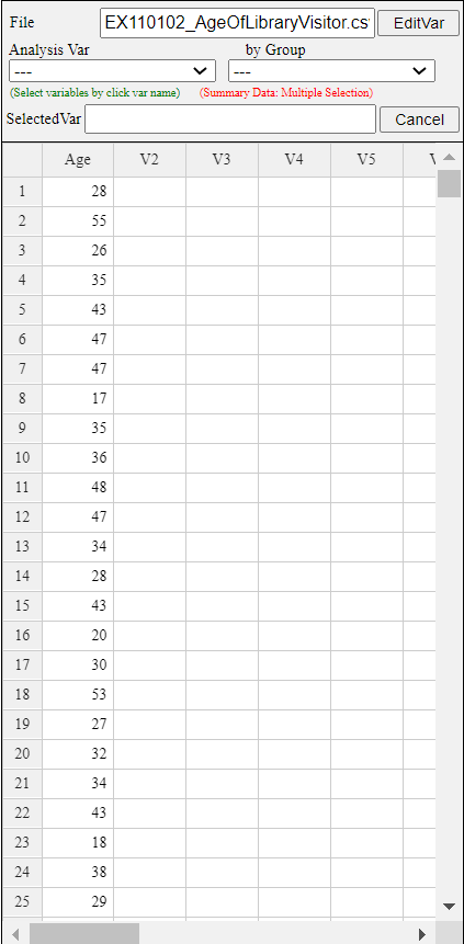
Example 11.1.2 Ages of 30 people who visited a library in the morning are as follows. Test the hypothesis that the population is normally distributed at the significance level of 5%.
Answer
Age is a continuous variable, but you can make a frequency distribution by dividing possible values into intervals as we studied in histogram of Chapter 3. It is called a categorization of the continuous data.
Let's find a frequency table which starts at the age of 10 with the interval size of 10. The histogram of 『eStat』 makes this frequency table easy to obtain.
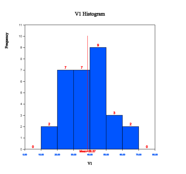
If you enter the data as shown in <Figure 11.1.3>, click the histogram icon and select Age from the variable selection box, then the histogram as <Figure 11.1.4> will appear.

If you specify 'start interval' as 10 and 'interval width' as 10 in the options window below the histogram, the histogram of <Figure 11.1.4> is adjusted as <Figure 11.1.5>. If you click [Frequency Table] button, the frequency table as shown in <Figure 11.1.6> will appear in the Log Area. The designation of interval size can be determined by a researcher.
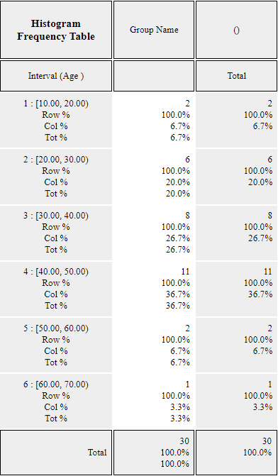
Since the normal distribution is a continuous distribution defined at \(-\infty \lt x \lt \infty\) , the frequency table of <Figure 11.1.6> can be written as follows:
| Interval id | Interval | Observed frequency |
|---|---|---|
| 1 | \( X < 20 \) | 2 |
| 2 | \(20 \le X < 30\) | 6 |
| 3 | \(30 \le X < 40\) | 8 |
| 4 | \(40 \le X < 50\) | 11 |
| 5 | \(50 \le X < 60\) | 2 |
| 6 | \( X \ge 60 \) | 1 |
The frequency table of sample data as Table 11.1.2 can be used to test the goodness of fit whether the sample data follows a normal distribution using the chi-square distribution. The hypothesis of this problem is as follows:
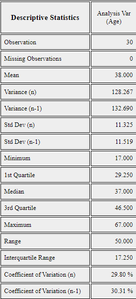
This hypothesis does not specify what a normal distribution is and therefore, the population mean \(\mu\) and the population variance \(\sigma^2\) should be estimated from sample data. Pressing the 'Basic Statistics' icon on the main menu of 『eStat』 will display a table of basic statistics in the Log Area, as shown in <Figure 11.1.7>. The sample mean is 38.000 and the sample standard deviation is 11.519.
Hence, the above hypothesis can be written in detail as follows:
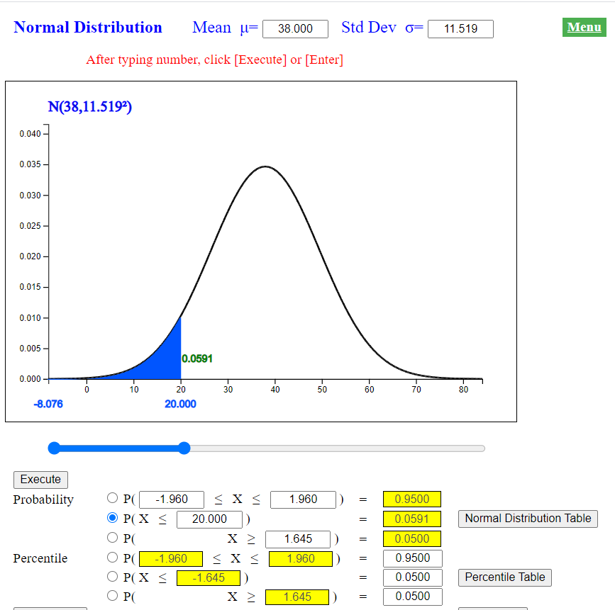
In order to find the expected frequency of each interval when \(\small H_0\) is true, the expected probability of each interval is calculated first using the normal distribution \(\small N(38.000, 11.519^2 )\) as follows. The normal distribution module of 『eStatU』 makes it easy to calculate this probability of an interval. At the normal distribution module of 『eStatU』, enter the mean of 38.000 and the standard deviation of 11.519. Click the second radio button of P(X < x) type and enter 20, then press the [Execute] button to calculate the probability as shown in <Figure 11.1.8>.
Similarly you can calculate the following probabilities.
Expected frequency can be calculated by multiplying the sample size of 30 to the expected probability of each interval obtained above. The observed frequencies, expected probabilities, and expected frequencies for each interval can be summarized as the following table.
| Interval id | Interval | Observed frequency | Expected probability | Expected frequency |
|---|---|---|---|---|
| 1 | \( X < 20 \) | 2 | 0.059 | 1.77 |
| 2 | \(20 \le X < 30\) | 6 | 0.185 | 5.55 |
| 3 | \(30 \le X < 40\) | 8 | 0.325 | 9.75 |
| 4 | \(40 \le X < 50\) | 12 | 0.282 | 8.46 |
| 5 | \(50 \le X < 60\) | 2 | 0.121 | 3.63 |
| 6 | \( X \ge 60 \) | 1 | 0.028 | 0.84 |
Since the expected frequencies of the 1st and 6th interval are less than 5, the intervals should be combined with adjacent intervals for testing the goodness of fit using the chi-square distribution as Table 11.1.4. The expected frequency of the last interval is still less than 5, but, if we combine this interval, there are only three intervals, we demonstrate the calculation as it is. Note that, due to computational error, the sum of the expected probabilities may not be exactly equal to 1 and the sum of the expected frequencies may not be exactly 30 in Table 11.1.4.
| Interval id | Interval | Observed frequency | Expected probability | Expected frequency |
|---|---|---|---|---|
| 1 | \( X < 30 \) | 8 | 0.244 | 7.32 |
| 2 | \(30 \le X < 40\) | 8 | 0.325 | 9.75 |
| 3 | \(40 \le X < 50\) | 11 | 0.282 | 8.48 |
| 4 | \( X \ge 50 \) | 3 | 0.149 | 4.47 |
| Total | 30 | 1.000 | 30.00 |
The test statistic for the goodness of fit test is as follows:
Since the number of intervals is 4, \(k\) becomes 4, and \(m\)=2, because two population parameters \(\mu\) and \(\sigma^2\) are estimated from the sample data. Therefore, the critical value is as follows:
The observed test statistic is less than the critical value, we can not reject the null hypothesis that the sample data follows \(\small N(38.000, 11.519^2 )\) .
Test result can be verified using [Categorical: Goodness of Fit Test] in 『eStatU』. In the Input box that appears by selecting the module, enter the data for 'Observed Frequency' and 'Expected Probability' in Table 11.1.4, as shown in <Figure 11.1.9>. After entering the data, select the significance level and press the [Execute] button to calculate the 'expected frequency' and produce a chi-square test result as in <Figure 11.1.10>.
[]
Data of 30 otter lengths can be found at the following location of 『eStat』.
Test the hypothesis that the population is normally distributed at the significance level of 5% using 『eStat』.
11.2 Testing Hypothesis for Contingency Table
[presentation] [video]
11.2.1 Independence Test
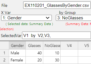
Example 11.2.1 In order to investigate whether college students who are wearing glasses are independent by gender, a sample of 100 students was collected and its contingency table was prepared as follows:
| Wear Glasses | No Glasses | Total | |
|---|---|---|---|
| Men | 40 | 10 | 50 |
| Women | 20 | 30 | 50 |
| Total | 60 | 40 | 100 |
Answer

| Wear Glasses | No Glasses | Total | |
|---|---|---|---|
| Men | 30 | 20 | 50 |
| Women | 30 | 20 | 50 |
| Total | 60 | 40 | 100 |
[]
| Variable A | Variable B | \(B_1\) | \(B_2\) | \(\cdots\) | \(B_c\) | Total |
|---|---|---|---|---|---|
| \(A_1\) | \(p_{11}\) | \(p_{12}\) | \(\cdots\) | \(p_{1c}\) | \(p_{1\cdot}\) |
| \(A_2\) | \(p_{21}\) | \(p_{22}\) | \(\cdots\) | \(p_{2c}\) | \(p_{2\cdot}\) |
| \(\cdots\) | \(\cdots\) | \(\cdots\) | \(\cdots\) | \(\cdots\) | \(\cdots\) |
| \(A_r\) | \(p_{r1}\) | \(p_{r2}\) | \(\cdots\) | \(p_{rc}\) | \(p_{r\cdot}\) |
| Total | \(p_{\cdot 1}\) | \(p_{\cdot 2}\) | \(\cdots\) | \(p_{\cdot c}\) | 1 |
| Variable A | Variable B | \(B_1\) | \(B_2\) | \(\cdots\) | \(B_c\) | Total |
|---|---|---|---|---|---|
| \(A_1\) | \(O_{11}\) | \(O_{12}\) | \(\cdots\) | \(O_{1c}\) | \(T_{1\cdot}\) |
| \(A_2\) | \(O_{21}\) | \(O_{22}\) | \(\cdots\) | \(O_{2c}\) | \(T_{2\cdot}\) |
| \(\cdots\) | \(\cdots\) | \(\cdots\) | \(\cdots\) | \(\cdots\) | \(\cdots\) |
| \(A_r\) | \(O_{r1}\) | \(O_{r2}\) | \(\cdots\) | \(O_{rc}\) | \(T_{r\cdot}\) |
| Total | \(T_{\cdot 1}\) | \(T_{\cdot 2}\) | \(\cdots\) | \(T_{\cdot c}\) | n |
| Variable A \ Variable B | \(B_1\) | \(B_2\) | \(\cdots\) | \(B_c\) |
|---|---|---|---|---|
| \(A_1\) | \(E_{11} = T_{1\cdot} \times \frac {T_{\cdot 1}}{n}\) | \(E_{12} = T_{1\cdot} \times \frac {T_{\cdot 2}}{n}\) | \(\cdots\) | \(E_{1c} = T_{1\cdot} \times \frac {T_{\cdot c}}{n}\) |
| \(A_2\) | \(E_{21} = T_{2\cdot} \times \frac {T_{\cdot 1}}{n}\) | \(E_{22} = T_{2\cdot} \times \frac {T_{\cdot 2}}{n}\) | \(\cdots\) | \(E_{2c} = T_{2\cdot} \times \frac {T_{\cdot c}}{n}\) |
| \(\cdots\) | \(\cdots\) | \(\cdots\) | \(\cdots\) | \(\cdots\) |
| \(A_r\) | \(E_{r1} = T_{r\cdot} \times \frac {T_{\cdot 1}}{n}\) | \(E_{r2} = T_{r\cdot} \times \frac {T_{\cdot 2}}{n}\) | \(\cdots\) | \(E_{rc} = T_{r\cdot} \times \frac {T_{\cdot c}}{n}\) |
This test statistic follows approximately a chi-square distribution with \((r-1)(c-1)\) degrees of freedom. Therefore, the decision rule to test the hypothesis with significance level of \(\alpha\) is as follows: $$ \text{'If}\quad \chi_{obs}^2 = \sum_{i=1}^{r} \sum_{j=1}^{c} \frac {(O_{ij} - E_{ij} )^2} {E_{ij}} \gt \chi_{(r-1)(c-1); α}^2,\; \text{then reject}\;\; H_0' $$
Hypothesis:
i.e., \(p_{ij} = p_{i·} \cdot p_{·j}, i=1,2, ... , r, \;\; j=1,2, ... , c\)
Decision Rule:
$$
\text{‘If}\quad \chi_{obs}^2 = \sum_{i=1}^{r} \sum_{j=1}^{c} \frac {(O_{ij} - E_{ij} )^2} {E_{ij}} \gt \chi_{(r-1)(c-1); α}^2,\; \text{then reject}\;\; H_0 ’
$$
where \(r\) is the number of attributes of row variable and \(c\) is the number of attributes of column variable.
\(\clubsuit\) If an expected frequency of a cell is smaller than 5, the cell is combined with adjacent cell for analysis.
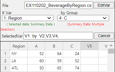
Example 11.2.2 A market research institute surveyed 500 people on how three beverage products (A, B and C) are preferred by region and obtained the following contingency table.
| Region \ Beverage | A | B | C | Total |
|---|---|---|---|---|
| New York | 52 | 64 | 24 | 140 |
| Los Angels | 60 | 59 | 52 | 171 |
| Atlanta | 50 | 65 | 74 | 189 |
| Total | 162 | 188 | 150 | 500 |
Answer

\(\small\qquad H_1\): Region and beverage preference are not independent.
\(\qquad ( \frac{162}{500}, \frac{88}{500}, \frac{50}{500} )\)
\(\small\qquad E_{11} = 140 \times \frac{162}{500} = 45.36, \quad E_{12} = 140 \times \frac{188}{500} = 52.64, \quad E_{13} = 140 \times \frac{150}{500} = 42.00\) \(\small\qquad E_{21} = 171 \times \frac{162}{500} = 55.40, \quad E_{22} = 171 \times \frac{188}{500} = 64.30, \quad E_{23} = 171 \times \frac{150}{500} = 51.30\) \(\small\qquad E_{31} = 189 \times \frac{162}{500} = 61.24, \quad E_{32} = 189 \times \frac{188}{500} = 71.06, \quad E_{33} = 189 \times \frac{150}{500} = 56.70\)
\(\qquad \chi_{obs}^2 = \sum_{i=1}^3 \sum_{j=1}^3 \; \frac{(O_{ij} - E_{ij} )^2 }{E_{ij}} = \frac{(52 -45.36)^2}{45.36} + \frac{(60-55.40)^2}{55.40} + \cdots + \frac{(74-56.70)^2}{56.70} \) = 19.822
\(\qquad \chi_{(r-1)(c-1); α}^2 = \chi_{(3-1)(3-1); 0.05}^2 = \chi_{4; 0.05}^2 \) = 9.488
[]
| TV View \ Reading | High | Low | Total |
|---|---|---|---|
| High | 40 | 18 | 58 |
| Low | 31 | 11 | 42 |
| Total | 71 | 29 | 100 |
11.2.2 Homogeneity Test
[presentation] [video]
| Score \ Grade | Freshman | Sophomore | Junior | Senior |
|---|---|---|---|---|
| A | - | - | - | - |
| B | - | - | - | - |
| C | - | - | - | - |
| D | - | - | - | - |
\(\qquad H_0\): Distributions of several populations for a categorical variable are homogeneous.
\(\qquad H_1\): Distributions of several populations for a categorical variable are not homogeneous.
The test statistic for the homogeneity test is the same as the independence test as follows: $$ \chi_{obs}^2 = \sum_{i=1}^{r} \sum_{j=1}^{c} \frac {(O_{ij} - E_{ij} )^2} {E_{ij}} $$ Here \(r\) is the number of attributes of row variable and \(c\) is the number of populations.
Hypothesis:
\(H_1\): Distributions of several populations for a categorical variable are not homogeneous.
Decision Rule: $$ \text{‘If}\quad \chi_{obs}^2 = \sum_{i=1}^{r} \sum_{j=1}^{c} \frac {(O_{ij} - E_{ij} )^2} {E_{ij}} \gt \chi_{(r-1)(c-1); α}^2,\; \text{then reject}\;\; H_0 ’ $$ Here \(r\) is the number of attributes of row variable and \(c\) is the number of populations.
\(\clubsuit\) If an expected frequency of a cell is smaller than 5, the cell is combined with adjacent cell for analysis.
Example 11.2.3 In order to investigate whether viewers of TV programs are different by age for three programs (A, B and C), 200, 100 and 100 samples were taken separately from the population of young people(20s), middle-aged people (30s and 40s), and older people (50s and over) respectively. Their preference of the program were summarized as follows. Test whether TV program preferences vary by age group at the significance level of 5%.
| TV Program \ Age Group | Young | Middle Aged | Older | Total |
|---|---|---|---|---|
| A | 120 | 10 | 10 | 140 |
| B | 30 | 75 | 30 | 135 |
| C | 50 | 15 | 60 | 125 |
| Total | 200 | 100 | 100 | 400 |
Answer
The hypothesis of this problem is as follows:
\(\quad \small H_1\): TV program preferences for different age groups are not homogeneous.
Proportions of the number of samples for each age group are as follows:
Therefore, the expected frequencies of each program when is true are as follows:
If two variables are independent, these proportions should be kept in each region. Hence, the expected frequencies in each region can be calculated as follows:
The chi-square test statistic and critical value are as follows:
\(\qquad \chi_{obs}^2 = \sum_{i=1}^3 \sum_{j=1}^3 \; \frac{(O_{ij} - E_{ij} )^2 }{E_{ij}} = \frac{(120-70)^2}{70} + \frac{(10-35)^2}{35} + \cdots + \frac{(60-31.25)^2}{31.25} \) = 180.495
\(\qquad \chi_{(r-1)(c-1); α}^2 = \chi_{(3-1)(3-1); 0.05}^2 = \chi_{4; 0.05}^2 \) = 9.488
Since \(\chi_{obs}^2\) is greater than the critical value, \(\small H_0\) is rejected. TV programs have different preferences for different age groups.
| Evaluation \ Training | Typing training | No training | Total |
|---|---|---|---|
| Good | 48 | 12 | 60 |
| Normal | 39 | 26 | 65 |
| Low | 13 | 62 | 75 |
| Total | 100 | 100 | 200 |