Chapter 13. Time Series Analysis
CHAPTER OBJECTIVES
In this chapter, we study data observed over time, time series, and introduce about:
--- What is time series analysis and what are the types of time series models?
--- How to smooth a time series.
--- How to transform a time series.
--- Prediction method using regression model.
--- Prediction method using exponential smoothing model.
--- Prediction method for seasonal time series.
We will be mainly focused on descriptive methods and simple models, and discussion of the Box-Jenkins model and other theoretical models will not be discussed.
13.1 What is Time Series Analysis?
Time series refers to data recorded according to changes in time. In general, observations are made at regular time intervals such as year, season, month, or day, and this is called a
discrete time series. There may be time series that are continuously observed, but this book will only deal with the analysis of discrete time series.
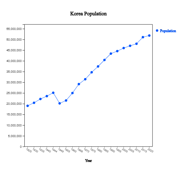
An example of a discrete time series is the population of Korea as shown in [Table 13.1.1]. This data is from the census conducted every five years in Korea from 1925 to 2020 (except for 1944 and 1949).
[Table 13.1.1] Population of Korea
| Year |
Population |
1925
1930
1935
1940
1944
1949
1955
1960
1966
1970
1975
1980
1985
1990
1995
2000
2005
2010
2015
2020
|
19020030
20438108
22208102
23547465
25120174
20166756
21502386
24989241
29159640
31435252
34678972
37406815
40419652
43390374
44553710
45985289
47041434
47990761
51069375
51829136
|
As shown in the table above, it is not easy to understand the overall shape of the time series displayed in numbers. The first step in time series analysis is to observe the time series by drawing a time series plot with the X axis as time and the Y axis as time series values. For example, the time series plot of the total population in Korea is shown in <Figure 13.1.1>.

<Figure 13.1.1>Time Series of Korea Population
|
Observing this figure, Korea's population has an overall increasing trend, but the population decreased sharply
in 1944-1949 due to World War II. It can be seen that the population expanded rapidly after the Korean war in 1953
and slowed since 1990. It can also be seen that the growth has slowed further in the last 10 years. By observing
the time series in this way, trends, change points, and outliers can be observed, which is helpful in selecting an analysis model or method suitable for the data.
Time series that we frequently encounter include monthly sales of department stores and companies, daily composite stock index, annual crop production, yearly export and import time series, and yearly national income and economic growth rate, and so on.
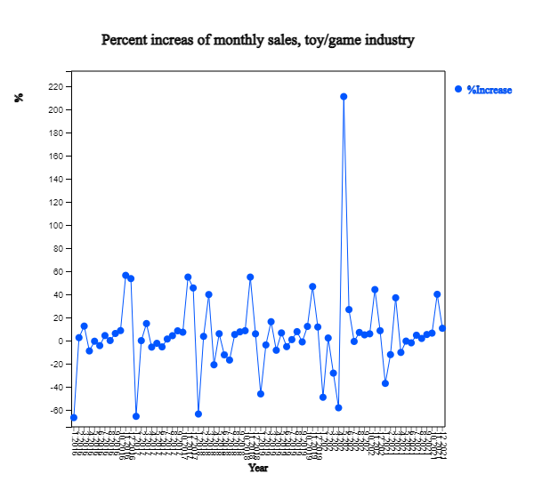
[Table 13.1.2] shows the percent increase in monthly sales of the US toy/game industry for the past 6 years, and <Figure 13.1.2> is a plot of this time series. As it is the rate of change from the previous month, it can be observed that it is seasonal data showing a large increase in November and December every year, moving up and down based on 0. However, May 2020 is an extreme with an increase rate of 211% unlike other years. For time series, you can better examine the characteristics of the data by converting the raw time series into the rate of change.
[Table 13.1.2] Percent Increase, Monthly Sales of Toy/Game in US(%) (Source: Bureau of Census, US)
| Year.month |
Percent Increase |
2016.01
2016.02
2016.03
2016.04
2016.05
2016.06
2016.07
2016.08
2016.09
2016.10
2016.11
2016.12
2017.01
2017.02
2017.03
2017.04
2017.05
2017.06
2017.07
2017.08
2017.09
2017.10
2017.11
2017.12
2018.01
2018.02
2018.03
2018.04
2018.05
2018.06
2018.07
2018.08
2018.09
2018.10
2018.11
2018.12
2019.01
2019.02
2019.03
2019.04
2019.05
2019.06
2019.07
2019.08
2019.09
2019.10
2019.11
2019.12
2020.01
2020.02
2020.03
2020.04
2020.05
2020.06
2020.07
2020.08
2020.09
2020.10
2020.11
2020.12
2021.01
2021.02
2021.03
2021.04
2021.05
2021.06
2021.07
2021.08
2021.09
2021.10
2021.11
2021.12
|
-66.7
2.5
12.5
-9.0
-0.6
-4.4
4.3
0.0
6.1
8.6
56.4
53.6
-65.6
-0.1
14.7
-5.7
-2.4
-5.5
1.3
4.2
8.4
7.2
54.9
45.5
-63.6
3.6
39.8
-21.0
5.9
-12.4
-16.9
5.2
7.5
8.5
54.9
5.8
-46.2
-3.8
16.3
-8.4
6.6
-5.3
0.8
7.7
-1.2
12.2
46.7
11.7
-49.1
2.2
-28.2
-58.2
211.1
26.8
-0.8
7.0
4.9
5.8
44.1
8.5
-37.1
-12.2
37.0
-10.3
-0.5
-2.0
4.6
1.8
5.2
6.4
40.0
10.6
|

<Figure 13.1.2>Percent Increase, Monthly Sales of Toy/Game in US(%)
|
Most time series have four components: trend, seasonal, cycle, and other irregular factors.
Trend is a case in which a time series has a certain trend, such as a line or a curved shape
as time elapses, and there are various types of trends. Trends can be understood as a consumption behavior,
population variations, and inflation that appear in time series over a long period of time.
Seasonal factors are short-term and regular fluctuation factors that exist quarterly, monthly,
or by day of the week. Time series such as monthly rainfall, average temperature, and ice cream sales
have seasonal factors. Seasonal factors generally have a short cycle, but fluctuations when the cycle
occurs over a long period of time rather than due to the season is called a cycle factor. By observing
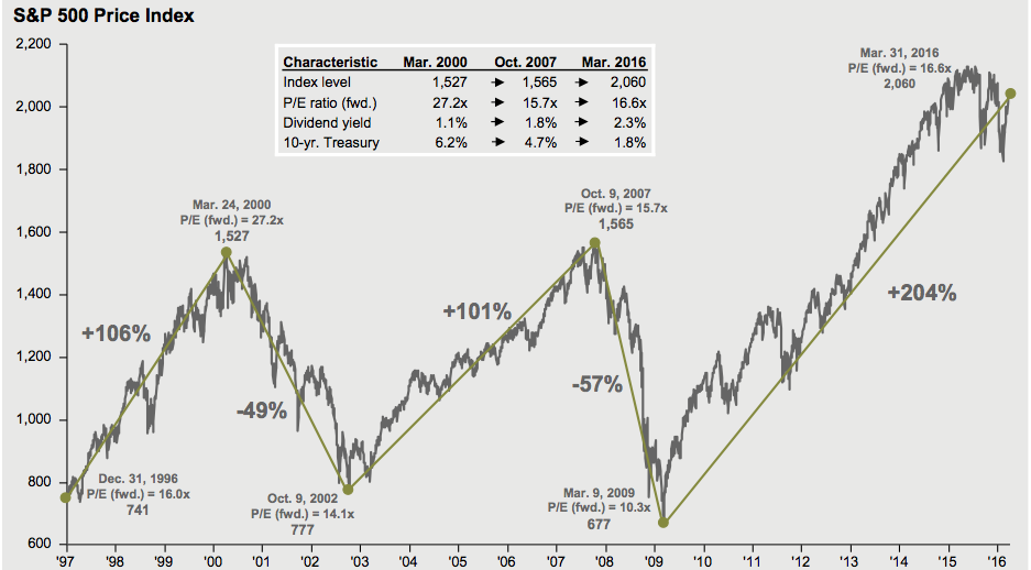
these cyclical factors, it is possible to predict the boom or recession of a periodic economy. <Figure 13.1.3> shows the US S&P 500 Index from 1997 to 2016, and a six-year cycle can be observed.

<Figure 13.1.3>] US S&P500 Index (1997- 2016)
|
Other factors that cannot be explained by trend, season, or cyclical factors are called irregular
or random factors, which refer to variable factors that appear due to random causes regardless of regular movement over time.
13.1.1 Time Series Model
By observing the time series, you can predict how this time series will change in the future by building a time series model that fits the probabilistic characteristics of this data. Because the time series observed in reality has a very diverse form, the time series model is also very diverse, from simple to very complex. In general, time series models for a single variable can be divided into the following four categories.
A. Regression Model
A model that explains data or predicts the future by expressing a time series in the form of
a function related to time is the most intuitive and easy to understand model. That is,
when a time series is an observation of a random variable, \(Y_1 , Y_2 , ... , Y_n\),
it is expressed as the following model:
$$
Y_t \;=\; f(t) \;+\; \epsilon _ t , \,\, t=1,2, ... , n
$$
Here \(\epsilon_t\) is the error of the time series that cannot be explained by a function \(f(t)\).
In general \(\epsilon_t\) is assumed independent, \(E(\epsilon_t ) = 0\) , and
\(Var(\epsilon_t ) = \sigma^2)\) which is called a white noise. For example, the following model
can be applied to a time series in which the data is horizontal or has a linear trend.
\( \qquad \text{Horizontal:} \qquad Y_t \;=\; \mu \;+\; \epsilon _ t \)
\( \qquad \text{Linear Trend:}\quad Y_t \;=\; a \;+\; b\, t \;+\; \epsilon _ t \)
B. Decomposition Model
The model that decomposes the time series into four factors, i.e., trend(\(T_t\)), cycle(\(C_t\)),
seasonal(\(S_t\)), and irregular(\(I_t\)), is an analysis method that has been used for a long time based on empirical facts. It can be divided into additive model and multiplicative model.
\( \qquad \text{Additive Model:} \qquad \qquad Y_t \;=\; T_t \;+\; C_t \;+\; S_t \;+\; I_t \)
\( \qquad \text{Multiplicative Model:}\qquad Y_t \;=\; T_t \;\times\; C_t \;\times\; S_t \;\times \; I_t \)
Here \(T_t\), \(C_t\), \(S_t\) are deterministic function, \(I_t\) is a random variable.
If we take the logarithm of a multiplicative model, it becomes an additive model.
If the number of data is not enough, the cycle factor can be omitted in the model.
C. Exponential Smoothing Model
Time series data are often more related to recent data than to past data. The above two types of models are models that do not take into account the relationship between the past time series data and the recent time series data. Models using moving averages and exponential smoothing are often used to explain and predict data using the fact that time series forecasting is more related to recent data.
D. Box-Jenkins ARIMA Model
The above models are not methods that can be applied to all types of time series, and the analyst selects and applies them according to the type of data. Box and Jenkins presented the following general ARIMA model that can be applied to all time series of stationary or nonstationary type as follows:
$$
Y _{t} \,=\, \mu \,+\, \phi_{1} \, Y _{t-1} \,+\, \phi _{2} \, Y_{t-2} \,+\, \cdots \,+\, \epsilon _{t} \,+\, \theta _{1} \, \epsilon _{t-1} \,+\, \theta _{2} \, \epsilon _{t-2} \,+\, \cdots
$$
The ARIMA model considers the observed time series as a sample extracted from a population time series, studies the probabilistic properties of each model, and establishes an appropriate time series model through parameter estimation and testing. For the ARIMA model, autocorrelation coefficients between time lags are used to identify a model. The ARIMA model is beyond the scope of this book, so interested readers are encouraged to consult the bibliography.
In the above time series model, the regression model and ARIMA model are systematic models based on statistical theory, and the decomposition model and exponential smoothing model are methods based on experience and intuition. In general, regression models using mathematical functions and models using decomposition are known to be suitable for predicting slow-changing time series, whereas exponential smoothing and ARIMA models are known to be effective in predicting very rapidly changing time series.
For all time series models, it is impossible to predict due to sudden changes. And because time series has so many different forms, it cannot be said that one time series model is always superior to another. Therefore, rather than applying only one model to a time series, it is necessary to establish and compare several models, combine different models, or make an effort to determine the final model by combining opinions of experts familiar with the time series.
13.1.2 Evaluation of Time Series Model
Let the time series be the observed values of the random variables \(Y_1 , Y_2 , ... , Y_n\)
and \(\hat Y_1 , \hat Y_2 , ... , \hat Y_n\) be the values predicted by the model.
If the model agrees exactly, the observed and predicted values are the same, and the model
error \(\epsilon_t\) is zero. In general, it is assumed that the error \(\epsilon_t\)’s of
the time series model are independent random variables which follow the same normal
distribution with a mean of 0 and a variance of \(\sigma^2\). The accuracy of a time series
model can be evaluated using residual, \(Y_t \,-\, {\hat Y}_t\), which is a measure by
subtracting the predicted value from the observed value. In general, the following mean squared error (MSE) is commonly used for the accuracy of a model and the smaller the MSE value, the more appropriate the predicted model is judged.
$$
{MSE} \,=\, \frac{ \sum_{t=1}^n \, ( Y_t\,-{\hat Y}_t \,)^{2} } {n}
$$
The mean square error is used as an estimator for the variance \(\sigma^2\) of the error \(\epsilon_t\).
Since MSE can have a large value, the root mean squared error (RMSE) is often used.
$$
{RMSE} \,=\, \sqrt{MSE }
$$
13.2 Smoothing of Time Series
Original time series data can be used to make a time series model by observing trends, but in many cases,
time series can be observed after smoothing to unerstand better. In a time series such as stock price, it is often difficult to find a trend because of temporary or short-term fluctuations due to accidental coincidences or cyclical factors. In this case, smoothing techniques are used as a method to effectively grasp the overall long-term trend by removing temporary or short-term fluctuations. The centered moving average method and the exponential smoothing method are widely used.
13.2.1 Centered Moving Average
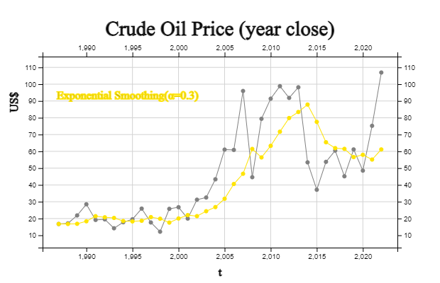
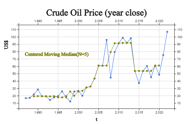
The time series in [Table 13.2.1] is the world crude oil price based on the closing price every year from 1987 to 2022. Looking at <Figure 13.2.1>, it can be seen that the short-term fluctuations in the time series are large. However, causes such as oil shocks are short-term and not continuous, so if we are interested in the long-term trend of gasoline consumption, it would be more effective to look at the fluctuations caused by short-term causes.
[Table 13.2.1] Price of Crude Oil (End of Year Price, US$) and 5-point Centered Moving Average
| Year |
Price of Oil |
5-point Centered Moving Average |
1987
1988
1989
1990
1991
1992
1993
1994
1995
1996
1997
1998
1999
2000
2001
2002
2003
2004
2005
2006
2007
2008
2009
2010
2011
2012
2013
2014
2015
2016
2017
2018
2019
2020
2021
2022
|
16.74
17.12
21.84
28.48
19.15
19.49
14.19
17.77
19.54
25.90
17.65
12.14
25.76
26.72
19.96
31.21
32.51
43.36
61.06
60.85
95.95
44.60
79.39
91.38
98.83
91.83
98.17
53.45
37.13
53.75
60.46
45.15
61.14
48.52
75.21
106.95
|
---
---
20.666
21.216
20.630
19.816
18.028
19.378
19.010
18.600
20.198
21.634
20.446
23.158
27.232
30.752
37.620
45.798
58.746
61.164
68.370
74.434
82.030
81.206
91.920
86.732
75.882
66.866
60.592
49.988
51.526
53.804
58.096
67.394
---
---
|
[ : . ]
<Figure 13.2.1> Price of Crude Oil, Smoothing and Filtering
The N-point centered moving average of a time series refers to the average of N data
from a single point in time. For example, in crude oil price data, the value of the
five-point moving average for a specific year is the average of the data for two years
before the specific year, that year, and the data for the next two years. Expressed as
an expression, if \(M_t\) is a moving average in time \(t\), the 5-point centered moving
average is as follows:
$$
M_t = \frac{Y_{t-2} \,+\, Y_{t-1} \,+\, Y_{t} \,+\, Y_{t+1} \,+\, Y_{t+2} } {5 }
$$
For example, the 5-point centered moving average for 1989 is as follows.
\(\qquad M_{1989} \,=\, \frac {Y_{1987} + Y_{1988} +Y_{1989} + Y_{1990} + Y_{1991} } {5 } \)
\( \qquad \qquad \quad =\, \frac {16.74 + 17.12 + 21.84 + 28.48 + 19.15} {5} \,=\, 20.6660 \)
[Table 13.2.2] shows the values of all 5-points centered moving averages obtained in this way and <Figure 13.2.1> is the graph of 5-points moving average. Note that the moving averages for the first two years and the last two years cannot be obtained here. It can be seen that the graph of the moving average is better for grasping the long-term trend than the graph of the original data because short-term fluctuations are removed.
The choice of a value N for the N-point moving average is important. A large value of N
will provide a smoother moving average, but it has the disadvantage of losing more points
at both ends and insensitive to detecting important trend changes. On the other hand,
if you choose small N, you will lose less data at both ends, but you may not be able
to get the smoothing effect because you will not sufficiently eliminate short-term fluctuations.
In general, try a few values N to reflect important changes that should not be missed,
while achieving a smoothing effect and balancing the points not to lose too much at both ends.
If the value of N is an even number, there is a difficulty in obtaining a central moving average
with the same number of data on both sides of the base year. For example, the center of the
four-point moving average from 1987 to 1990 is between 1988 and 1989. If you denote this as
\(M_{1988.5}\), it can be calculated as follows:
\( \qquad M_{1988.5} \,=\, \frac {Y_{1987} + Y_{1988} +Y_{1989} + Y_{1990} } {4 }
\,=\, \frac {16.74 + 17.12 + 21.84 + 28.48 } {4} \,=\, 21.045 \)
The 4-point moving average obtained in this way is called a non-central 4-points moving average.
In the case of this even number N, the non-central moving average does not match the observation
year of the original data, which is inconvenient. In the case of this even number N, it is
calculated as the average of the noncentral moving average values of two adjacent non-central
moving averages. In other words, the central four-point moving average in 1989 is the average
of \(M_{1988.5}\) and \(M_{1989.5}\) as follows:
\( \qquad M_{1989} \,=\, \frac {M_{1988.5} \,+\, M_{1989.5} } {2 } \,=\, \frac {21.0450 \,+\, 21.6475 } {2} \,=\, 21.3463 \)
If the time series is quarterly or monthly, a 4-point central moving average or a 12-point central moving average is an average of one year, so it is often used to observe data without seasonality.
13.2.2 Exponential Smoothing
3-point moving average can be considered the weighted average of three data with each weight
\(\frac{1}{3}\) as follows:
$$
M_t \,=\, \frac{Y_{t-1} \,+\, Y_{t} \,+\, Y_{t+1} } {3 } \,=\, \frac{1}{3}Y_{t-1} \,+\, \frac{1}{3}Y_{t} \,+\, \frac{1}{3}Y_{t+1}
$$
When the weights are \(w_1 , w_2 , ... , w_n\), the weighted moving average \(M_t\) of the
time series is defined as follows:
$$
M_t \,=\, \sum_{i=1}^{n} w_i Y_{i}
$$
where \(n\) is the number of data, \(w_i \ge 0\) and \(\sum_{i=1}^{n} w_i = 1 \).
Various weighted averages with different weights can be used depending on the purpose.
Among them, a smoothing method that gives more weight to data closer to the present and
smaller weights as it is farther from the present is called exponential smoothing.
The exponential smoothing method is determined by an exponential smoothing constant \(\alpha\)
that has a value between 0 and 1. The exponentially smoothed data \(E_t\) is calculated as follows:
\( \qquad E_{1} \,=\, \alpha \,Y_{1} \,+\, (1- \alpha)\, E_{0} \)
\( \qquad E_{2} \,=\, \alpha \,Y_{2} \,+\, (1- \alpha)\, E_{1} \)
\( \qquad E_{3} \,=\, \alpha \,Y_{3} \,+\, (1- \alpha)\, E_{2} \)
\( \qquad \cdots \)
\( \qquad E_{t} \,=\, \alpha \,Y_{t} \,+\, (1- \alpha)\, E_{t-1} \)
Here, an initial value \(E_{0}\) is required, and \(Y_1\) is usually used a lot, and the average
value of the data can also be used. The exponentially smoothed value \(E_t\) at the point in time
\(t\) gives weight \(\alpha\) to the current data, and the \(1-\alpha\) weight to the previous
smoothed data is given. The exponentially smoothed value \(E_t\) can be represented with
the original data \(Y_t\) as follows:
$$
E_t \,=\, \alpha Y_t + \alpha (1-\alpha) Y_{t-1} + \alpha(1-\alpha)^2 Y_{t-2} + \cdots + \alpha(1-\alpha)^{t-2} Y_2 + \alpha(1-\alpha)^{t-1} Y_1 + (1-\alpha)^t E_0
$$
Therefore, the exponential smoothing method uses all data from the present and the past, but gives
the current data the highest weight α, and gives a lower weight as the distance from the present time increases.
Exponential smoothing of the crude oil price in [Table 13.2.1] with the initial value
\(E _{1986} = Y _{1987} \) and exponential smoothing constant \(\alpha\) = 0.3 is as follows.
\( \qquad E_{1986} \,=\, E_{1987} = 16.74 \)
\( \qquad E_{1987} \,=\, 0.3 \,Y_{1987} \,+\, (1- 0.3)\, E_{1986} \,=\, (0.3)(16.74)+(0.7)(16.74)=16.74 \)
\( \qquad E_{1988} \,=\, 0.3 \,Y_{1988} \,+\, (1- 0.3)\, E_{1987} \,=\, (0.3)(17.12)+(0.7)(16.74)=16.854 \)
All data exponentially smoothed with \(\alpha\) = 0.3 are given in [Table 13.2.2]. It can be seen that,
in the exponential smoothing method, there is no loss of data at both ends, unlike the moving average method.
The crude oil price time series and exponentially smoothed data are shown in <Figure 13.2.2>.
It can be seen that the smoothed data are not significantly different from the original data.
If the value of \(\alpha\) is small, more weight is given to the past data than to the present,
making it less sensitive to sudden changes in the present data. Conversely, the closer the value of
\(\alpha\) is to 1, that is, the more weight is given to the current data, the more the smoothed data
resembles the original data, and the smoothing effect disappears.
[Table 13.2.2] Price of Crude Oil and Exponential Smoothing with α =0.3
| Year |
Price of Oil |
Exponential Smoothing
α=0.3 |
1987
1988
1989
1990
1991
1992
1993
1994
1995
1996
1997
1998
1999
2000
2001
2002
2003
2004
2005
2006
2007
2008
2009
2010
2011
2012
2013
2014
2015
2016
2017
2018
2019
2020
2021
2022
|
16.74
17.12
21.84
28.48
19.15
19.49
14.19
17.77
19.54
25.90
17.65
12.14
25.76
26.72
19.96
31.21
32.51
43.36
61.06
60.85
95.95
44.60
79.39
91.38
98.83
91.83
98.17
53.45
37.13
53.75
60.46
45.15
61.14
48.52
75.21
106.95
|
16.740
16.854
18.350
21.389
20.717
20.349
18.501
18.282
18.659
20.832
19.877
17.556
20.017
22.028
21.408
24.348
26.797
31.766
40.554
46.643
61.435
56.385
63.286
71.714
79.849
83.443
87.861
77.538
65.416
61.916
61.479
56.580
57.948
55.120
61.146
74.888
|
13.2.3 Filtering by Moving Median
The N-point
centered moving median of a time series refers to the median of N data from a single point
in time \(t\). For example, in crude oil price data, the value of a five-point moving median for a specific
year is the median of data for two years before a certain year, that year, and data for two years thereafter.
If data are denoted by \(Y_{t-2} ,Y_{t-1} , Y_{t} , Y_{t+1} , Y_{t+2} \), and the data are sorted from
smallest to largest, and expressed as \(Y_{(t-2)} ,Y_{(t-1)} , Y_{(t)} , Y_{(t+1)} , Y_{(t+2)} \),
the median value is \(Moving Median_t \,=\, Y_{(t)}\).
For example, the 5-point central moving median in 1989 for crude oil prices in [Table 13.2.3] is as follows:
\(\qquad MovingMedian_{1989} \,=\, median \{ Y_{1987} , Y_{1988} ,Y_{1989} , Y_{1990} , Y_{1991} \} \)
\(\qquad \qquad \qquad \qquad \qquad \;\;\;=\, median \{16.74, 17.12 , 21.84 , 28.48,19.15 \} \,=\, 19.15 \)
[Table 13.2.3] and <Figure 13.2.3> show all the five-point moving median values obtained in this way and their graphs. Note that the moving median for the first two years and the last two years are not available here. Because the centered moving medians remove extreme values, it is called a filtering and the time series is much smoother than the original data.
[Table 13.2.3] Price of Crude Oil and 5-point Centered Moving Median
| Year |
Price of Oil |
5-point Centered Moving Median |
1987
1988
1989
1990
1991
1992
1993
1994
1995
1996
1997
1998
1999
2000
2001
2002
2003
2004
2005
2006
2007
2008
2009
2010
2011
2012
2013
2014
2015
2016
2017
2018
2019
2020
2021
2022
|
16.74
17.12
21.84
28.48
19.15
19.49
14.19
17.77
19.54
25.90
17.65
12.14
25.76
26.72
19.96
31.21
32.51
43.36
61.06
60.85
95.95
44.60
79.39
91.38
98.83
91.83
98.17
53.45
37.13
53.75
60.46
45.15
61.14
48.52
75.21
106.95
|
19.15
19.49
19.49
19.15
19.15
19.49
17.77
17.77
19.54
25.76
19.96
25.76
26.72
31.21
32.51
43.36
60.85
60.85
61.06
79.39
91.38
91.38
91.83
91.83
91.83
53.75
53.75
53.45
53.75
53.75
60.46
61.14
|
If the value of N is an even number, there is a difficulty in obtaining the central moving median having
the same number of data on both sides of the base year. For example, the center of the four-point moving
median from 1987 to 1990 is between 1988 and 1989. If you denote this as \(Median_{1988.5}\), it can be
calculated as follows:
\(\qquad MovingMedian_{1988.5} \,=\, median \{Y_{1987} , Y_{1988} , Y_{1989} , Y_{1990} \} \)
\(\qquad \qquad \qquad \qquad \qquad \quad \;\;=\, median \{16.74 , 17.12 , 21.84 , 28.48 \} \,=\, \frac {17.12 +21.84} {2} = 19.48 \)
The 4-point moving median obtained in this way is called the non-central 4-point moving median.
As such, the non-central moving average in the case of this even number N does not match the
observation year of the original data, which is inconvenient. In the case of this even number,
it is calculated as the average of the values of the two non-central moving medians that are
adjacent to each other. In other words, the central four-point moving median in 1989 is the mean of
\(MovingMedian_{1988.5}\) and \(MovingMedian_{1989.5}\).
13.3 Transformation of Time Series
Time series can be viewed by drawing the raw data directly, but in order to examine various characteristics, change in percentage increase or decrease is examined, and an index that is a percentage with respect to base time is alse examined. In addition, in order to examine the relation of the previous data, it is compared with a time lag or converted into horizontal data using the difference. When the variance of the time series increases with time, it is sometimes converted into a form suitable for applying the time series model by using logarithmic, square root, or Box-Cox transformation.
13.3.1 Percentage Change
A. Percent Change
In a time series, you can examine the increase or decrease of a value, but you can easily observe
the change by calculating the percentage increase or decrease. When the time series is expressed as
\(Y_1 , Y_2 , ... , Y_n\) , the percentage increase or decrease \(P_t\) compared to the previous data is as follows.
$$
P_{t} \,=\, \frac {Y _{t} - Y_{t-1}} {Y_{t-1}} \times 100 , \quad t=2,3, ... , n
$$
[Table 13.3.1] shows the number of houses in Korea from 2010 to 2020, and <Figure 13.3.1> shows
the percentage increase or decrease compared to the previous data. Looking at this rate of change,
it can be easily observed that the original time series has an overall increasing trend, but the rate
of change of the previous year has many changes. In other words, it can be observed that there was a
2.23% increase in the number of houses in 2014 compared to the previous year, and a 2.48% increase
in the number of houses in 2018 as well.
\(\qquad P_{2014} \,=\, \frac{19161.2 - 18742.1} {18742.1} \times 100 \,=\, 2.23 \)
[Table 13.3.1] Number of Houses in Korea and Percent Change (Korea National Statistical Office, unit 1000)
| Year |
Number of Houses |
% change |
2010
2011
2012
2013
2014
2015
2016
2017
2018
2019
2020
|
17738.8
18082.1
18414.4
18742.1
19161.2
19559.1
19877.1
20313.4
20818.0
21310.1
21673.5
|
1.93
1.83
1.77
2.23
2.07
1.62
2.19
2.48
2.36
1.70
|
[ : ]
<Figure 13.3.1> Number of Houses in Korea and Transformation
B. Simple Index
Another way to use percentages to easily characterize changes over time is to calculate an index number.
An
index \(I_t\) is a number that indicates the change over time of a time series. The index number
\(Index_t\) of a time series at a certain point in time is the percentage of the total time series data
for a predetermined time point \(t_0\) called the base period.
$$
Index_{t} \,=\, \frac {Y _{t}} {Y_{t_0}} \times 100 , \quad t=1,2,..., n
$$
The most commonly used indices in the economic field are the price index and the quantity index.
For example, the consumer price index is a price index indicating the price change of a set of goods
that can reflect the total consumer price, and the index indicating the change in total electricity
consumption every year is the quantity index. There are several methods of calculating the index,
which are broadly divided into simple index number when the number of items represented by the index is one, and composite index number when there are several as in the consumer price index.
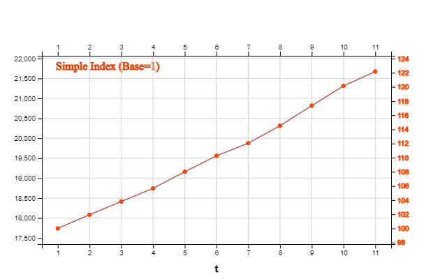
[Table 13.3.2] is a simple index for the number of houses in Korea from 2010 to 2020, with the base
time being 2010. If you look at the figure for the index, you can see that in this case, there is no significant change from the original time series and trend. It can be seen that there is a 22.18% increase in the number of houses in 2020 compared to 2010.
\(\qquad Index_{2020} \,=\, \frac{Y _{2020}} {Y_{2010}} \times 100 \,=\, \frac{21673.5} {17738.8} \times 100 \,=\, 122.18 \)
[Table 13.3.2] Simple Index of Number of Houses in Korea (Korea National Statistical Office, unit 1000)
| Year |
Number of Houses |
Simple Index
Base: 2010 |
2010
2011
2012
2013
2014
2015
2016
2017
2018
2019
2020
|
17738.8
18082.1
18414.4
18742.1
19161.2
19559.1
19877.1
20313.4
20818.0
21310.1
21673.5
|
100.00
101.94
103.81
105.66
108.02
110.26
112.05
114.51
117.36
120.13
122.18
|
C. Composite Index
Composite index is a method in which the change in price or quantity of several goods is set at a specific time point as the base period, and then the data at each time point is calculated as a percentage value compared to the base period. An example of the most used composite index is the consumer price index, which reflects price fluctuations of about 500 products in Korea that affect consumer prices. Other commonly used composite indices include the comprehensive stock index, which examines the price fluctuations of all listed stocks traded in the stock market.
For the composite index, a weighted composite index that is calculated by weighting the price of each
product with the quantity consumed is often used. When calculating such a weighted composite index,
the case where the quantity consumption at the base time is used as a weight is called the
Laspeyres method, and the case where the quantity consumption at the current time is used
as the weight is called the Paasche method. In general, the Laspeyres method of weighted composite index is widely used, and the consumer price index is a representative example. The price index of the Paasche method is used when the consumption of goods used as weights varies greatly over time, and can be used only when the consumption at each time point is known. It is expensive to examine the quantity consumption at each point in time.
Assuming that \(P_{1t} , \cdots , P_{kt} \) are the prices of \(k\) number of products at the time point \(t\),
and \(Q_{1t_0} , \cdots , Q_{kt_0} \) are the quantities of each product consumpted at the base time,
the formula for calculating each composite index is as follows:
\( \qquad \text{Laspeyres Index:} \quad Index_t \,=\, \frac { Q_{1t_0} P_{1t} + \cdots + Q_{kt_0} P_{kt} } {Q_{1t_0} P_{1t_0}+ \cdots + Q_{kt_0} P_{kt_0} } \times 100 \)
\( \qquad \text{Paasche Index:} \qquad Index_t \,=\, \frac { Q_{1t} P_{1t} + \cdots + Q_{kt} P_{kt} } {Q_{1t} P_{1t_0} + \cdots + Q_{kt} P_{kt_0} } \times 100 \)
The data in [Table 13.3.3] shows the price and quantity of three metals by month in 2020.
[Table 13.3.3] Composite Index of three Metal Prices($/ton) and Production Quantity (ton)
Month |
Copper
Price Quantity |
Metal
Price Quantity |
Lead
Price Quantity |
Laspeyres Paasche |
1
2
3
4
5
6
7
8
9
10
11
12
|
1361.6 100.7
1399.0 95.1
1483.6 104.0
1531.6 95.6
1431.2 103.3
1383.8 106.9
1326.8 95.9
1328.8 96.7
1307.8 95.7
1278.4 89.1
1354.2 100.5
1305.2 96.9
|
213 4311
213 4497
213 5083
213 5077
213 5166
213 4565
213 4329
213 4057
213 3473
213 3739
213 3817
213 3694
|
530.0 46.1
520.0 47.0
529.0 51.0
540.0 23.0
531.0 26.5
580.0 13.5
642.8 27.4
602.6 25.8
513.6 20.5
480.8 24.6
528.4 21.5
462.2 27.9
|
100.00 100.00
100.31 100.28
101.13 101.01
101.63 101.35
100.65 100.57
100.42 100.27
100.16 99.98
100.00 99.87
99.43 99.38
99.01 99.07
99.92 99.92
99.18 99.21
|
In [Table 13.3.3], the Laspeyres index for the data for February with January as the base time is as follows.
\( \qquad Index_t \,=\, \frac { Q_{1t_0} P_{1t} + \cdots + Q_{kt_0} P_{kt} } {Q_{1t_0} P_{1t_0}+ \cdots + Q_{kt_0} P_{kt_0} } \times 100
\,=\, \frac {(100.7)(1399.0)+(4311)(213)+(46.1)(520) } {(100.7)(1361.6)+(4311)(213)+(46.1)(530) } \,=\, 100 .31 \)
Similarly, Paasche index is as follows:
\( \qquad Index_t \,=\, \frac { Q_{1t} P_{1t} + \cdots + Q_{kt} P_{kt} } {Q_{1t} P_{1t_0} + \cdots + Q_{kt} P_{kt_0} } \times 100
\,=\, \frac {(95.1)(1399.0)+(4497)(213)+(47.0)(520) } {(95.1)(1361.6)+(4497)(213)+(47.0)(530) } \,=\, 100.28 \)
In [Table 13.3.3], it can be seen that the production quantity of iron and lead in the last 4 quarters is significantly different from the production quantity in January, which is the base time. In this way, when the quantity fluctuates greatly and the quantity at each time is known, the Pasche index can be said to be the best index because it appropriately reflects the price change at that time.
13.3.2 Time Lag and Difference
A. Time Lag
In a time series, current data can usually be related to past data.
Lag means a transformation for
comparing data of the present time and observation values at one time point or a certain past time point.
That is, when the observed time series is \(Y_1 , Y_2 , ... , Y_n\), the time series with lag 1 becomes
\( - , Y_1 , Y_2 , ... , Y_{n-1}\) . Note that, in case of lag k, there are no data for the first \(k\) number than the original data.
The correlation coefficient between the time lag data and the raw data is called the
autocorrelation coefficient.
If the average of time series is \(\small \overline Y\) , the k-lag autocorrelation \(r_k\) is defined as follows:
$$ \small
r_k = \frac { \sum_{t = k+1}^ n (Y_t - \overline Y ) (Y_{t-k} - \overline Y ) } { \sum _{t =1}^n (Y_t - \overline Y )^2 }, \quad k=0, 1, 2, ..., n-1
$$
\(r_1 , r_2 , ... , r_k \) are called an autocorrelation function and are used to determine a time series model.
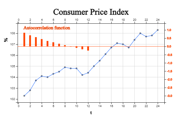
[Table 13.3.4] shows the monthly consumer price index for the past two years and time lag 1 to 12 for this data, and the autocorrelation coefficients are shown in [Table 13.3.5]. <Figure 13.3.3> shows the original time series and the autocorrelation function.
[Table 13.3.4] Monthly Consumer Price Index and Time Lag 1, Lag 2, ... Lag 12
| t |
Year.Month |
CPI |
lag 1 |
lag 2 |
... |
lag 12 |
1
2
3
4
5
6
7
8
9
10
11
12
13
14
15
16
17
18
19
20
21
22
23
24
|
2020.01
2020.02
2020.03
2020.04
2020.05
2020.06
2020.07
2020.08
2020.09
2020.10
2020.11
2020.12
2021.01
2021.02
2021.03
2021.04
2021.05
2021.06
2021.07
2021.08
2021.09
2021.10
2021.11
2021.12
|
102.3
102.8
103.7
104.1
104.0
104.3
104.5
104.9
104.8
104.8
104.2
104.4
105.0
105.5
106.1
106.7
107.1
107.0
106.7
107.4
108.0
107.7
107.8
108.3
|
102.3
102.8
103.7
104.1
104.0
104.3
104.5
104.9
104.8
104.8
104.2
104.4
105.0
105.5
106.1
106.7
107.1
107.0
106.7
107.4
108.0
107.7
107.8
|
102.3
102.8
103.7
104.1
104.0
104.3
104.5
104.9
104.8
104.8
104.2
104.4
105.0
105.5
106.1
106.7
107.1
107.0
106.7
107.4
108.0
107.7
|
...
|
102.3
102.8
103.7
104.1
104.0
104.3
104.5
104.9
104.8
104.8
104.2
104.4
|
[Table 13.3.5] Autocorrelation Function
| time |
autocorrelation |
1
2
3
4
5
6
7
8
9
10
11
|
0.8318
0.6772
0.5651
0.4479
0.3333
0.2547
0.1647
0.0755
-0.0143
-0.0854
-0.1737
|
B. Differencing
Since the price index in [Table 13.3.4] has a linear trend, a model for this trend can be built,
but in some cases, a model can be created by changing the time series to a horizontal trend.
The way to transform a linear trend into a horizontal trend is to use a
differencing.
When the time series is \(Y_1 , Y_2 , ... , Y_n \), the first order difference \(▽ Y_t\) is as follows:
$$
▽ Y_t \,=\, Y_t \,-\, Y_{t-1}, \quad t=2,3,...,n
$$
If the raw data is a linear trend, the first-order differencing of time series is a horizontal
time series because it means a change in slope. If we make differencing on the first-order difference \(▽ Y_t\),
it becomes the second-order difference as follows:
$$
▽^2 Y_t \,=\, ▽Y_t \,-\, ▽Y_{t-1} \,=\, ( Y_t \,-\, Y_{t-1} ) - ( Y_{t-1} \,-\, Y_{t-2}), \quad t=3,4,...,n
$$
If the raw data has a trend with a quadratic curve, the second-order differencing of time series becomes a horizontal time series.
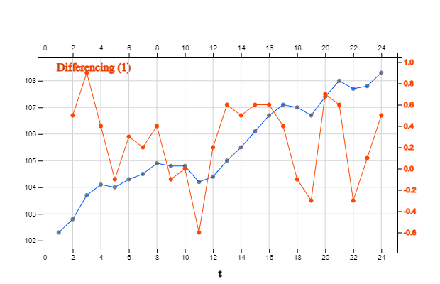
<Figure 13.3.4> shows the first order differencing of [Table 13.3.4] time series and it becomes horizontal series.
13.3.3 Mathematical Transformation
If the original data of the time series is used as it is, modeling may not be easy or it may not satisfy various assumptions. In this case, we can fit the model we want by performing an appropriate functional transformation, such as log transformation. The functions commonly used for mathematical transformations are as follows.
\( \qquad \text{Log function } \qquad\qquad \qquad W = log(Y) \)
\( \qquad \text{Square root function} \qquad\quad W = \sqrt(Y) \)
\( \qquad \text{Square function } \qquad\quad \qquad W = Y^2 \)
\( \qquad \text{Box-Cox Transformation} \quad \; W = \frac {Y^p - 1 }{p} \) if p ≠ 0, else log(Y)
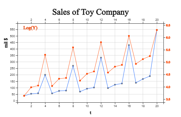
[Table 13.3.6] is a toy company's quarterly sales, and <Figure 13.3.5> is a
diagram of this data. It is a seasonal data by quarter, but, as time goes on,
dispersion of sales increases over time. It is not easy to apply a time series model
to data with this increasing dispersion over time. In this case, log transformation
\(W = log(Y)\) can reduce the dispersion as time increases, as shown in
<Figure 13.3.5>, so that a model can be applied. After predicting by applying
the model to log-transformed data, exponential transformation \(Y = exp(W)\) is
performed again to predict the raw data.
[Table 13.3.6] Quarterly Sales of a Toy Company (unit million $)
| time |
Year |
Sales |
1
2
3
4
5
6
7
8
9
10
11
12
13
14
15
16
17
18
19
20
|
2017 Quarter 1
2017 Quarter 2
2017 Quarter 3
2017 Quarter 4
2018 Quarter 1
2018 Quarter 2
2018 Quarter 3
2018 Quarter 4
2019 Quarter 1
2019 Quarter 2
2019 Quarter 3
2019 Quarter 4
2020 Quarter 1
2020 Quarter 2
2020 Quarter 3
2020 Quarter 4
2021 Quarter 1
2021 Quarter 2
2021 Quarter 3
2021 Quarter 4
|
38.0
53.6
57.5
200.0
56.5
75.8
78.3
269.7
70.2
92.7
101.8
332.6
97.3
123.7
132.9
429.4
138.3
167.6
189.9
545.9
|
The square root transform is used for a similar purpose to the log transform, and the square transform can be used when the variance decreases with time. The Box-Cox transform is a general transformation.
13.4 Regression Model and Forecasting
If there is a trend factor that shows a continuous increase or decrease in the time series,
the regression model learned in Chapter 12 can be applied. For example, if the time series
shows a linear trend, the linear regression model is applied with the time series as
the observation values of the random variable \(Y_1 , Y_2 , ... , Y_n\) and time
as 1, 2, ... , \(n\) as follows.
$$
Y_t \,=\, \beta_0 \,+\, \beta_1 t \,+\, \epsilon_t
$$
Here \(\epsilon_t \) is the error term with mean 0 and variance \(\sigma^2\).
A characteristic of the linear model is that it increases by a slope \(\beta_1\)
of a certain magnitude over time.
When the estimated regression coefficients are \(\beta_0 , \beta_1\), the validity test
of the linear regression model is the same as the method described in Chapter 12.
The standard error of estimate and coefficient of determination are often used.
In a linear trend model, \(\sigma\) represents the degree to which observations
can be scattered around the estimated regression line at each time point. As an estimate
of this \(\sigma\), the following standard error is used.
$$
s \,=\, \sqrt { \frac{1} {n-2} \sum_{t=1}^n ( Y_t - {\hat Y}_t )^2 }
$$
A smaller standard error \(s\) value indicates that the observed values are close to
the estimated regression line, which means that the regression line model is well fitted.
The coefficient of determination is the ratio of the regression sum of squares, RSS, which is explained out of the total sum of squares, TSS.
$$
R^2 \,=\, \frac{RSS}{TSS}
$$
The value of the coefficient of determination is always between 0 and 1, and the closer the value is to 1, the more dense the samples are around the regression line, which means that the estimated regression equation explains the observations well.
As explained in Chapter 12, since it is difficult to determine the absolute criteria for adequacy of
the standard error or the coefficient of determination, a hypothesis test is used to determine whether
the trend parameter \(\beta_1\) is zero or not.
\(\small \qquad \text{Hypothesis: } \qquad \,\, H_0 : \beta_1 = 0, H_1: \beta_1 \ne 0\)
\(\small \qquad \text{Test statistic:} \qquad t_{obs} = \frac {{\hat \beta}_1 } { SE ({{\hat \beta}_1 }) } \) ,
Here, \( SE( \hat{ \beta_1} ) \,=\, \frac{ s} { \sqrt { \sum_{i=1}^ n (i - \overline t )^2 } } \)
\(\small \qquad \text{Rejection region:} \quad If \,\; |t_{obs}| \,>\, t_{n-2,\alpha/2}, \,\,reject\,\, H_0 \) with significance level \(\alpha\)
If the null hypothesis \(H_0\) is not rejected, the model cannot be considered valid.
The assumption for error \(\epsilon_t\) is tested using the residual, which is the difference between the observed time series value and the predicted value which is called residual analysis. Residual analysis usually examines whether assumptions about error terms such as independence and equal variance between errors are satisfied by drawing a scatter plot of the residuals over time or a scatter plot of the residuals and predicted values. In the scatterplots, if the residuals do not show a specific trend around 0 and appear randomly, it means that each assumption is valid. To examine the normality assumption of the error term, draw a normal probability plot of the residuals, and if the points on the figure show the shape of a straight line, it is judged that the assumption of the normal distribution is appropriate.
If the linear regression model is suitable, the predicted value
\({\hat Y}_{t_0} \,=\, {\hat \beta}_0 \,+\, {\hat \beta}_1 \cdot t_0 \) at the time point \(t_0\)
can be interpreted as a point estimate for the mean of the random variable \(Y_{t_0}\) at the time point,
and the confidence interval for the mean of \({\hat Y}_{t_0}\) at this time \(t_0\) is as follows:
$$\small
{\hat Y}_{t_0} \,±\, t_{n-2,\alpha/2} \cdot SE ({\hat Y}_{t_0} ) \;\; where \;\, SE ( {\hat Y}_{t_0} ) \,=\, s \cdot \sqrt { \frac{1}{n} + \frac {(t_0 - \overline t )^2} { \sum_{i=1}^n (i - \overline t )^2 } }
$$
If the trend is in the form of a quadratic, cubic or higher polynomial, the following multiple linear regression model can be assumed.
\( \qquad \text{Quadratic} \qquad Y_t = \beta_0 + \beta_1 \cdot t + \beta_2 \cdot t^2 + \epsilon _t \)
\( \qquad \text{Cubic} \qquad \qquad Y_t = \beta_0 + \beta_1 \cdot t + \beta_2 \cdot t^2 + \beta_3 \cdot t^3 + \epsilon _t \)
The prediction method is similar to the above simple linear regression model.
If the trend is not a polynomial model as above, the following model can also be considered.
\( \qquad \text{Square root} \qquad Y_t = \beta_0 + \beta_1 \cdot \sqrt{t} + \epsilon _t \)
\( \qquad \text{Log} \qquad \qquad \quad \; Y_t = \beta_0 + \beta_1 \cdot log(t) + \epsilon _t \)
These models are the same as the linear regression model if \(\sqrt{t}\) or \(log(t)\)
are replaced with the independent variable X in the simple linear regression and the prediction method is similar.
In addition, the function types to which the linear regression model can be applied by transformation are as follows.
\( \qquad \text{Power} \qquad \qquad Y _{t} = \beta_{0} \cdot t ^{\beta _{1}} + \epsilon _{t} \)
\( \qquad \text{Exponential} \quad \;\; Y_t = \beta_0 \cdot e^ {( \beta_1 t)} + \epsilon _t \)
In the case of these two models, the parameters should be estimated using the nonlinear regression model,
but if the error term is ignored, the linear model can be estimated approximately as follows:
\( \qquad \text{Power} \qquad \qquad log(Y_{t}) = log(\beta_{0}) +{\beta _{1}} \cdot log(t) \)
\( \qquad \text{Exponential} \quad \;\; log(Y_t) = log(\beta_0) + \beta_1 \cdot t \)
Korea's GDP from 1986 to 2021 is shown in [Table 13.4.1]. <Figure 13.4.1> shows the application of
three regression models to this data. Among these models, the quadratic model has the largest value of
\(r^2\) = 0.9591, so it can be said that the time series is the most suitable model. However, additional validation of the model is required.
[Table 13.4.1] GDP of Korea
| Year |
GDP (billion $) |
1991
1992
1993
1994
1995
1996
1997
1998
1999
2000
2001
2002
2003
2004
2005
2006
2007
2008
2009
2010
2011
2012
2013
2014
2015
2016
2017
2018
2019
2020
|
330.65
355.53
392.67
463.62
566.58
610.17
569.76
383.33
497.51
576.18
547.66
627.25
702.72
793.18
934.9
1053.22
1172.61
1047.34
943.67
1143.98
1253.16
1278.43
1370.8
1484.32
1465.77
1499.36
1623.07
1725.37
1651.42
1638.26
|
[ : ]
<Figure 13.4.1> Korea GDP data and regression model
13.5 Exponential Smoothing Model and Forecasting
When the time series moves in a trend, the future can be predicted well with the regression model. However, it may not be appropriate to predict a time series that is dynamically moving hourly, daily, etc. In this case, a moving average model or an exponential smoothing model can be used. The time series model is explained into two cases where the trend is stationary and linear.
13.5.1 Stationary Time Series
A time series is called stationary if the statistical properties such as mean, variance and covariance
are consistent over time. When a time series is the observed values of random variables
\(Y_1 , Y_2 , ... , Y_T\), a stationary time series is the following model that changes around
a constant value \(\mu \).
$$
Y_i \;=\; \mu \;+\; \epsilon_i , \quad i=1,2,..., T
$$
Here \(\mu\) is unknown parameter and \(\epsilon_i\) is an error term which is independent with mean 0 and variance \(\sigma^2\).
A. Single Moving Average Model
In a stationary time series model, the estimated value of \(\mu\), \(\hat \mu\), is the mean of the data. .
$$
{\hat \mu} \;=\; \frac{1}{T} \sum_{ i=1}^T Y_i
$$
Using this model, the prediction after \(\tau\) time points ahead at the current time \(T\) denoted
as \({\hat Y}_{T+\tau}\), is as follows:
$$
{\hat Y}_{T+\tau} \;=\; \hat \mu, \quad \tau=1,2,...
$$
It is called a
simple average model.
The simple average model uses all observations until the current time. However, the unknown
parameter \(\mu\) may shift slightly over time, so it would be reasonable to give more weight
to recent data than to past data for prediction. If a weight \(\frac{1}{N}\) is given to only
the most recent \(N\) observations at the present time \(T\) and the weight of the remaining
observations is set to 0, the estimated value of \(\mu\) is as follows.
$$
{\hat \mu} \;=\; \frac{1}{N} \sum_{ i=T-N+1}^T Y_i \;=\; \frac{1}{N} ( Y_{T-N+1} + Y_{T-N+2} + \cdots + Y_T )
$$
This is called a single moving average at the time point \(T\) and it is denoted by \(M_T\).
The single moving average means the average of the \(N\) observations adjacent to the time point \(T\).
Notice
that \(Y_1, Y_2 , ... , Y_T\) are independent of each other by assumption, but \(M_1, M_2 , ... , M_T\)
are not independent of each other, but are correlated.
The value of the single moving average varies depending on the size of \(N\). When the value of \(N\)
is large, it becomes insensitive to the fluctuations of the original time series, so it changes
gradually, and when the value of \(N\) is small, it becomes sensitive to fluctuations. Therefore,
when the fluctuation of the original time series is small, it is common to set the small value of \(N\),
and when the fluctuation is large, it is common to set the value of large \(N\).
Using the single moving average model at the time point \(T\), the predicted value and the mean
and variance of the predicted value at the time point \(T+\tau\) are as follows.
\(\qquad {\hat Y}_{T+\tau} \;=\; M_T , \quad \tau=1,2, ... \)
\(\qquad E( {\hat Y}_{T+\tau} ) \;=\; E(M_T ) \;=\; \mu \)
\(\qquad Var({\hat Y}_{T+\tau} )\;=\; Var(M_t ) \;=\; \frac{ \sigma ^2} {N } \)
When the single moving average model is used, the 95% confidence interval estimation of the
predicted value is approximately as follows.
\(\qquad {\hat{Y}} _{T+ \tau } \;±\; 1.96 \sqrt {Var( {\hat{Y}} _{T+ \tau } )} \)
\(\qquad M_{T} \;±\; 1.96 \sqrt{ \frac{MSE} {N} } \)
The monthly sales for the last two years of a furniture company are as shown in [Table 13.5.1],
and the residual between the raw data and the predicted value of one point in time was calculated
by obtaining a six-point moving average. <Figure 13.5.1> shows the time series for this.
This time series fluctuates up and down based on approximately 95, and such a time series is
called a stationary time series.
When \(N\) = 6, the moving average for the first 5 time points cannot be obtained.
The moving average at time 6 is as follows:
$$
M_6 \;=\; \frac{95+100+87+123+90+96} {6} \;=\; 98.50
$$
Therefore, one time prediction at time 6 becomes \({\hat Y}_{6+1} = 98.50 \) and the residual
at time 7 is as follows:
$$
e_{7} \;=\; Y_{7} \;-\; {\hat{Y}}_{6+1} \;=\; 75-98.50 \;=\; -23.50
$$
In the same way, the moving average of the remaining time points, the predicted values after one time point, and the residuals are as shown in [Table 13.5.1], so the mean square error is as follows:
$$
{ MSE} \;=\; \frac { \sum_{ i=7}^{ 24} ( Y_i \;-\; {\hat Y}_i )^{2} } {18} \;=\;331.22
$$
Sales for the next three months are the last moving average \(M_{24}\), and the 95% confidence
interval for the forecast is as follows:
\(\qquad {\hat Y}_{24+1} \;=\; {\hat Y}_{24+2} \;=\; {\hat Y}_{24+3} \;=\; M_{24} \;=\; 104.67 \)
\(\qquad M_T \;±\; 1.96 \sqrt \frac{MSE}{N } \)
\(\qquad 104.67 \;±\; 1.96 \sqrt \frac{331.22}{6} \)
\(\qquad [90.10, 119.23] \)
[Table 13.5.1] Montly Sales of a Furniture Company and 6-point Moving Average, One Time Forecast and Residuals
time
\(t\) |
Sales
(unit million $)
\(Y_t\) |
6-pt Moving
Average
\(M_t\) |
One Time
Forecast
\({\hat Y}_t\) |
Residual
\(e_t = Y_t - {\hat Y}_t\) |
1
2
3
4
5
6
7
8
9
10
11
12
13
14
15
16
17
18
19
20
21
22
23
24
|
95
100
87
123
90
96
75
78
106
104
89
83
118
86
86
112
85
101
135
120
76
115
90
92
|
98.50
95.17
91.50
94.67
91.50
91.33
89.17
96.34
97.67
94.34
95.67
95.00
98.00
100.84
106.50
104.84
105.34
106.17
104.67
|
98.50
95.17
91.50
94.67
91.50
91.33
89.17
96.34
97.67
94.34
95.67
95.00
98.00
100.84
106.50
104.84
105.34
106.17
|
-23.50
-17.17
14.50
9.33
-2.50
-8.33
28.83
-10.33
-11.67
17.67
-10.67
6.00
37.00
19.17
-30.50
10.17
-15.33
-14.17
|
[ : ]
<Figure 13.5.1> Montly Sales of a Furniture Company and 6-point Moving Average and One Time Forecast
※ Moving average at initial period
Since the \(N\)-point single moving average cannot be obtained before the time point \(N\),
the prediction model cannot be applied. When there are many time series, this may not be
a big problem, but when the number of data is small, it can affect the prediction. In order to
solve this problem, the moving average at initial period can be obtained as follows until
the time point \(N-1\).
\(\qquad t=1 \qquad \quad M_1 = Y_1 \)
\(\qquad t=2 \qquad \quad M_2 = \frac{Y_1 + Y_2 } {2} \)
\(\qquad \cdots \)
\(\qquad t=N-1 \quad M_{N-1} = \frac{Y_1 + Y_2 + \cdots + Y_{N-1} } {N - 1} \)
B. Single Exponential Smoothing Model
In the single moving average model, the same weight \(\frac{1}{N}\) is given to only the latest
\(N\) observations, and the previous observations are completely ignored by setting the weight to 0.
The
single exponential smoothing method compensates for the shortcomings of the moving average
model by assigning weights to all observations when predicting future values from past observations,
but giving more weight to recent data. This single exponential smoothing model uses the value of the
exponential smoothing method as the predicted value.
The single exponential smoothing model calculates the weighted average of the exponential
smoothing estimator \({\hat \mu}_{t-1} \) at the immediately preceding time point and the observation
value \(Y_t\) at the time point \(t\). Assuming that the exponential smoothing estimated value
at the time point \(t\) is \(S_t \;=\; {\hat \mu}_t \) and \(\alpha\) is a real number
between 0 and 1, the single exponential smoothing value \(S_t\) is defined as follows:
\(\qquad S_1 \;=\; \alpha \;Y_1 \;+\; (1-\alpha) S_0 \)
\(\qquad S_2 \;=\; \alpha \;Y_2 \;+\; (1-\alpha) S_1 \)
\(\qquad \cdots \)
\(\qquad S_t \;=\; \alpha \;Y_t \;+\; (1-\alpha) S_{t-1} \)
Here, \(\alpha\) is called the smoothing constant, and the single exponential smoothing value
\(S_t\) is the weighted average value given the weight \(\alpha\) of the most recent observation
\(Y_t\) and the weight (1-\(\alpha\)) of the exponential smoothing value \(S_{t-1}\) at the time \(t-1\).
You can better understand the meaning of exponential smoothing if you write down the recursive
equation as follows:
\(\qquad S_t \;=\; \alpha \;Y_t \;+\; (1-\alpha) S_{t-1} \)
\(\qquad \;=\; \alpha \; Y_t + (1- \alpha )\;( \alpha Y_{t-1} + (1- \alpha ) S_{t-2} ) \)
\(\qquad \;=\; \alpha Y_t + \alpha (1- \alpha ) Y_{t-1} + (1- \alpha )^2 S_{t-2} \)
\(\qquad \;=\; \alpha Y_t + \alpha (1- \alpha ) Y_{t-1} + \alpha(1- \alpha )^2 Y_{t-2} \;+\cdots\; + \alpha (1- \alpha )^{(t-1)} Y_1 +(1- \alpha )^t S_0 \)
In other words, for the single exponential smoothing value \(S_t\), the most recent observation
\(Y_t\) is given a weight \(\alpha\), and the next most recent observation is given \(\alpha(1-\alpha)\),
the next is \(\alpha(1-\alpha)^2\) and so on, a gradually smaller weight. Therefore,
if the size of \(\alpha\) is small, the current observation value is given a small weight,
and the exponential smoothing value is insensitive to the fluctuations of the time series.
if the size of \(\alpha\) is large, the current observation value is given a large weight,
and the exponential smoothing value is sensitive to the fluctuations of the time series.
In general, a value between 0.1 and 0.3 is often used as the value of \(\alpha\).
In order to obtain a single exponential smoothing value, an initial smoothing value
\(S_0\) is required, and the first observation value or the sample average of several
initial data or the overall sample average can be used. The exponential smoothing method
has the advantage of being less affected by extreme point or intervention than the ARIMA model
and easy to use, although the selection of the smoothing constant is arbitrary and
it is difficult to obtain a prediction interval.
The predicted value, average and variance of the predicted value at the time point \(T+\tau\) using the
single exponential smoothing model are as follows:
\(\qquad {\hat Y}_{T+\tau} \;=\;S_T \)
\(\qquad E( {\hat Y}_{T+\tau} )\;=\;E(S_T )\;=\; \mu \)
\(\qquad Var( {\hat{Y}}_{T+ \tau } )\;=\; Var(S_{T} )\;=\; \frac{\alpha } {2- \alpha } \sigma^{2} \)
Therefore, when the single exponential smoothing model is used, the 95% interval estimation in the predicted value is approximately as follows.
\(\qquad {\hat Y}_{T+\tau} \;±\; 1.96 \sqrt { Var ({\hat Y}_{T+\tau})} \)
\(\qquad S_{T} \;±\;1.96\; \sqrt { \frac{\alpha } {2- \alpha } MSE} \)
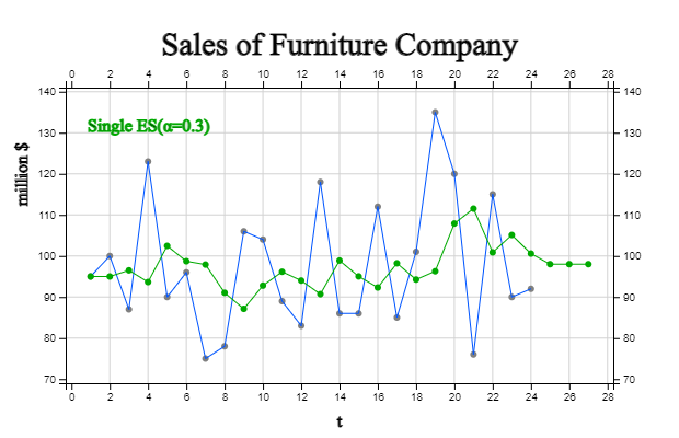
To the data of [Table 13.5.1], predict sales for the next three months by a single exponential
smoothing model with smoothing constant \(\alpha\) = 0.1. Lets use the first observed value
for the initial value of exponential smoothing, that is \(S_0 = Y_1 = 95\). The exponential smoothing value for the first three time series are as follows:
\(\qquad S_{1} \;=\;0.1\; \times \;Y _{1} \;+\;(1-0.1\;)\; \times \;S _{0} \;=\;\;0.1\; \times \;95\;+\;0.9\; \times \;95\;=\;95 \)
\(\qquad S_{2} \;=\;0.1\; \times\;Y_2 \;+\; (1-0.1\;)\;\times\; S_1 \;=\; \;0.1\;\times\;100\;+\;0.9 \;\times \;95 \;=\; 95.50 \)
\(\qquad S_{3} \;=\;0.1\; \times \;Y _{3} \;+\;(1-0.1\;)\; \times \;S _{2} \;=\;\;0.1\; \times \;87\;+\;0.9\; \times \;95.5\;=\;94.65 \)
\(\qquad \cdots \)
At each time point, the prediction after one point in time is as follows:
\(\qquad {\hat Y}_{0+1} \;=\; S_0 \;=\;95.00 \)
\(\qquad {\hat Y}_{1+1} \;=\; S_1 \;=\;95.00 \)
\(\qquad {\hat Y}_{2+1} \;=\; S_2 \;=\;95.50 \)
Hence the residuals using the above estimated values are as follows:
\(\qquad e_1 \;=\; Y_1\;-\;{\hat Y}_{0+1} \;=\; 95.00 - 95.00 \;=\; 0 \)
\(\qquad e_2 \;=\; Y_2\;-\;{\hat Y}_{1+1} \;=\; 100.00 - 95.00 \;=\; 5.00 \)
\(\qquad e_3 \;=\; Y_3\;-\;{\hat Y}_{2+1} \;=\; 87.00-95.50\;=\;-8.50 \)
In the same way, the single exponential smoothing of the remaining time points, the predicted values after one time point, and the residuals are as shown in [Table 13.5.2]. Therefore, the mean square error is as follows:
\(\qquad {MSE} \;= \; \frac{1}{24} \sum_{i=1}^{24} \; ( Y_i \;-{\hat Y}_i )^{2} \;=\;269.72 \)
In terms of mean square error, the MSE of the 6-point single moving average model is 331.22, so it can be said that the exponential smoothing model has better fit.
Sales for the next three months are the last moving average \(S_{24}\), and the 95% confidence interval for the forecast is as follows:
\(\qquad {\hat Y}_{24+1} \;=\; {\hat Y}_{24+2} \;=\; {\hat Y}_{24+3} \;=\; S_{24} \;=\; 98.66 \)
\(\qquad S_{T} \;±\; 1.96\; \sqrt { \frac{\alpha } {2- \alpha} } MSE \)
\(\qquad 98.66 \;±\; 1.96 \; \sqrt { \frac{0.1} {2-0.1} 269.72 } \)
\(\qquad [65.27, 132.05] \)
[Table 13.5.2] summarizes the above equations, and <Figure 13.5.2> shows the prediction after
one time point and the prediction for the next 3 months using the single exponential smoothing model with
\(\alpha\) = 0.1.
[Table 13.5.2] Exponential Smoothing with α = 0.1, One Time Forecast and Residual
time
\(t\) |
Sales
(unit million $)
\(Y_t\) |
Exponential
Smoothing
\(S_t\) |
One Time
Forecast
\({\hat Y}_t\) |
Residual
\(e_t = Y_t - {\hat Y}_t\) |
1
2
3
4
5
6
7
8
9
10
11
12
13
14
15
16
17
18
19
20
21
22
23
24
|
95
100
87
123
90
96
75
78
106
104
89
83
118
86
86
112
85
101
135
120
76
115
90
92
|
95.00
95.50
94.65
97.48
96.74
96.66
94.50
92.85
94.16
95.15
94.53
93.38
95.84
94.86
93.97
95.77
94.70
95.33
99.29
101.36
98.83
100.45
99.40
98.66
|
95.00
95.00
95.50
94.65
97.48
96.74
96.66
94.50
92.85
94.16
95.15
94.53
93.38
95.84
94.86
93.97
95.77
94.70
95.33
99.29
101.36
98.83
100.45
99.40
|
0.00
5.00
-8.50
28.35
-7.48
-0.74
-21.66
-16.50
13.15
9.84
-6.15
-11.53
24.62
-9.84
-8.86
18.03
-10.77
6.30
39.67
20.71
-25.36
16.17
-10.45
-7.40
|
※ Initial value of exponential smoothing
Since the initial exponential smoothing value \(S_0\) at the time point \(t=1\) cannot be obtained,
the following three methods are commonly used.
1) The first observation, i.e., \(S_0 \;=\; Y_1\)
2) Partial average using the initial \(n\) observation values, i.e.,
\(\qquad S_0 \;=\; \frac{1}{n} ({Y_1 + Y_2 + \cdots + Y_n }) \)
3) The mean up to the entire time point \(T\), i.e.,
\(\qquad S_0 \;=\; \frac{1}{T} ({Y_1 + Y_2 + \cdots + Y_T }) \)
※ Initial smoothing constant
The same smoothing constant \(\alpha\) can be applied to all time series, but the following
method is also used to reduce the effect of the initial value \(S_0\).
\(\qquad \alpha_t \;=\; \frac{1}{t} , \quad until \; \alpha_t \; reaches\; \alpha \)
13.5.2 Linear Trend Time Series
A. Double Moving Average Model
In the previous section, we examined that the single moving average model can be applied
to a stationary time series. What would happen if the single moving average model was applied
to a time series with a linear trend? That is, for a time series with a linear trend
\(Y_t \;=\; \beta_0 \;+\; \beta_1 \cdot t \;+\; \epsilon _t \), the \(N\)-point single moving average
at time \(T\) is as follows:
$$
M_T \;= \; \frac{1}{N} ( Y_{T-N+1} \;+\; Y_{T-N+2} \;+\; \cdots \;+\; Y_T )
$$
The expected value can be shown as follows:
$$
E(M_T) \;=\; \beta_0 + \beta_1 T - \frac{N-1} {2} \beta_1
$$
That is, in the case of a linear trend model, it can be seen that the single moving average \(M_t\)
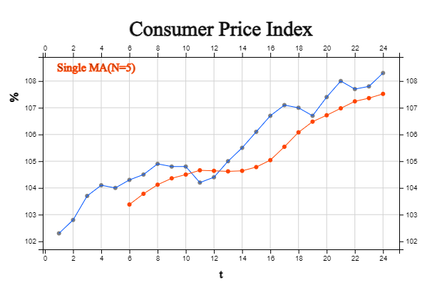
is biased by \(\frac{N-1}{2} \beta_1 \). For example, if the consumer price index with a linear trend
in [Table 13.5.3] is predicted after one point in time using the 5-point single moving average,
it is as shown in <Figure 13.5.3>. It can be seen that the predicted value using \(M_t\)
is under estimated value of the time series .
In the case of a linear trend, one way to eliminate the bias of the single moving average model
is the double moving average, which obtains the moving average again for the single moving average.
The \(N\)-point double moving average \(M_T^{(2)}\) at the time \(T\) and its expected value are
as follows:
$$
\begin{align}
M_T^{(2)} &\;=\; \frac{1}{N} (M_T \;+\; M_{T-1} \;+\; \cdots \;+\; M_{T-N+1}) \\
E(M_T^{(2)}) &\;=\; \beta_0 \;+\; \beta_1 T \;-\; (N-1) \beta_1
\end{align}
$$
Since \(E(M_T )\) and \(E(M_T ^{(2)} )\) have the same number of parameters, \(\beta_0 ,\;\beta_1 \)
can be estimated by solving the system of two equations as follows:
$$
\begin{align}
{\hat{\beta }}_{1} &\;=\; \frac{2}{N-1} \; (M_{T} \;-\; M_{T}^{(2)} ) \\
{\hat{\beta }}_{0} &\;=\; 2M_{T} \;-\; M_{T}^{(2)} \;-\; {\hat{\beta }}_{1} \;T\;
\end{align}
$$
Therefore, the predicted value at the time point \(T+\tau\) using the double moving average
at time \(T\) as follows:
$$
{\hat Y}_{T+\tau} \;=\; 2 M_T \;-\; {M_T ^{(2)}} \;+\; \tau \;\; (\frac {2}{N-1} ) \;\; (M_T\;-\; M_T^{(2)})
$$
Such a double moving average model can be said to be a kind of heuristic method. That is, although logical, it is not based on any optimization such as least squares method. However, it can be approximated by the least-squares method, which we will omit in this book.
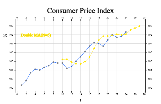
[Table 13.5.3] is a calculation table for predicting the consumer price index using the 5-point
double moving average model. Note that the third column is a 5-point single moving average \(M_T\),
but the single moving average cannot be calculated from time points 1 to 4. The fourth column
is the calculation of the 5-point double moving average \(M_t^{(2)}\), but the double moving average
cannot be calculated until 5 single moving averages have been calculated, that is, from time points
1 to 8. Using \(M_9\) and \(M_9^{(2)}\) to obtain the prediction after time 1 from time 9,
\({\hat Y}_{9+1}\) is as follows:
$$
\begin{align}
{\hat Y}_{9+1} &\;=\; 2M_9 \;- M_9^{(2)} \;+ 1 \;\; (\frac{2}{5-1}) \;\;(M_9\;-\;M_9 ^{(2)}) \\
&\;=\; 2 \times 104.50\;-104.028\;+1\;\; ( \frac{2}{5-1} ) \;\;(104.50\;-104.028)\;=\;105.2080
\end{align}
$$
The predicted values calculated in the same way are shown in the fifth column.
[Table 13.5.3] Double Moving Average of Consumer Price Index and One Time Forecast
time
\(t\) |
CPI
\(Y_t\) |
5-pt Single
Moving Average
\( M_t\) |
5-pt Double
Moving Average
\( M_t ^(2)\) |
One Time Forecast\({\hat Y}_{(t-1)+1}\) |
1
2
3
4
5
6
7
8
9
10
11
12
13
14
15
16
17
18
19
20
21
22
23
24
|
102.3
102.8
103.7
104.1
104.0
104.3
104.5
104.9
104.8
104.8
104.2
104.4
105.0
105.5
106.1
106.7
107.1
107.0
106.7
107.4
108.0
107.7
107.8
108.3
|
103.38
103.78
104.12
104.36
104.50
104.66
104.64
104.62
104.64
104.78
105.04
105.54
106.08
106.48
106.72
106.98
107.24
107.36
107.52
107.84
|
104.028
104.284
104.456
104.556
104.612
104.668
104.744
104.924
105.216
105.584
105.972
106.36
106.70
106.956
107.164
107.388
|
105.2080
105.2240
104.9160
104.7160
104.6820
104.9480
105.4840
106.4640
107.3760
107.8240
107.8420
107.9100
108.0500
107.9660
108.0540
|
B. Holt Double Exponential Smoothing Model
Holt proposed a model for a linear time series \(Y_t \;=\; \beta_0 \;+\; \beta_1 \cdot t \;+\; \epsilon_t \)
which uses a smoothing constant for the level and a smoothing constant for the trend. This is
called
Holt's linear trend exponential smoothing model or two-parameters double exponential
smoothing model. Let \({\hat b}_0 \) and \({\hat b}_1 \) be the initial values of the intercept
and slope, and \(\alpha\) be the smoothing constant of the level and \(\gamma\) is the smoothing
constant of the trend. The predicted values \({\hat Y}_t\), level \({\hat \beta}_0 (t)\) and
trend \({\hat \beta}_1 (t)\) are as follows:
$$
\begin{align}
& \text{Predicted value:} \quad {\hat Y}_t \;=\; {\hat \beta}_0 (t-1) + {\hat \beta}_1 (t-1) \\
& \text{Level:} \qquad\qquad \; {\hat \beta}_{0}(t) \;=\; \alpha Y_t + (1-\alpha) {\hat Y}_t \\
& \text{Trend:} \qquad\qquad {\hat \beta}_{1}(t) \;=\; {\gamma} \{ {\hat \beta}_0 (t) - {\hat \beta}_0 (t-1) \} + (1-\gamma) {\hat \beta}_1 (t-1)
\end{align}
$$
That is, the level is the weighted average of the current observed value \(Y_t\) and the predicted value
\({\hat Y}_t\), and the trend is the weighted average of the level difference
\({\hat \beta}_0 (t) - {\hat \beta}_0 (t-1) \) between the time points \(t\) and \((t-1)\) and
the trend \({\hat \beta}_1 (t-1) \) at the time point \((t-1)\). For this model, initial values
of level \({\hat \beta}_0 (0) \) and slope \({\hat \beta}_1 (0) \) are required and the intercept
and slope of the simple regression analysis of all observed values are widely used as initial estimates.
Similar to the single exponential smoothing model, a value between 0.1 and 0.3 is often used
to determine the smoothing constants \(\alpha\) and \(\gamma\).
The predicted values for the time point \(T+\tau\) at time \(T\) using the trend exponential
smoothing model are as follows:
$$
{\hat Y}_{T+\tau} \;=\; {\hat Y}_T + \tau {\hat \beta}_1 (T)
$$
Such a trend exponential smoothing model is also a kind of heuristic method. That is, although logical, it is not based on any optimization such as least squares method.
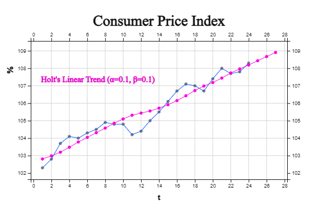
The result of simple linear regression model to all data in [Table 13.5.4] is as follows:
$$
{\hat{Y}}_{t} =102.574 \;+\; 0.2344 \;\;t
$$
[Table 13.5.4] is a calculation table for predicting the consumer price index with the Holt
double exponential smoothing model using this initial values. The third column is the predicted
value of the level \({\hat \beta}_0 (t) \), the fourth column is the trend \({\hat \beta}_ (t) \),
and the fifth column is the prediction \({\hat Y}_t = {\hat \beta}_0 (t-1) + {\hat \beta}_1 (t-1) \)
obtained one time after each time point. Therefore, the forecast of the consumer price index for
the next three months is as follows:
$$
\begin{align}
& t=25 \qquad {\hat{Y}} _{24+1} \;=\; {\hat{Y}} _{24} \;+\; 1\; \times {\hat{\beta}} _{1} (24)\;=\;108.19 +0.237\;=\;108.42 \\
& t=26 \qquad {\hat{Y}} _{24+2} \;=\; {\hat{Y}} _{24} \;+\; 2\; \times {\hat{\beta}} _{1} (24)\;=\;108.19 + 2 \times0.237\;=\;108.66 \\
& t=27 \qquad {\hat{Y}} _{24+3} \;=\; {\hat{Y}} _{24} \;+\; 3\; \times {\hat{\beta}} _{1} (24)\;=\;108.19 + 3 \times0.237\;=\;108.90
\end{align}
$$
[Table 13.5.4] Forecasting using Holt Double Exponential Smoothing Model of Consumer Price Index
time
\(t\) |
CPI
\(Y_t\) |
Constant
\( {\hat \beta}_0 (t)\) |
Trend
\( {\hat \beta}_1 (t)\) |
One Time Forecast\({\hat Y}_{(t-1)+1}\) |
0
1
2
3
4
5
6
7
8
9
10
11
12
13
14
15
16
17
18
19
20
21
22
23
24
|
102.3
102.8
103.7
104.1
104.0
104.3
104.5
104.9
104.8
104.8
104.2
104.4
105.0
105.5
106.1
106.7
107.1
107.0
106.7
107.4
108.0
107.7
107.8
108.3
|
102.57
102.76
102.97
103.25
103.54
103.80
104.07
104.33
104.61
104.85
105.07
105.20
105.33
105.50
105.70
105.93
106.20
106.49
106.75
106.96
107.21
107.50
107.73
107.95
108.20
|
0.234
0.229
0.227
0.232
0.239
0.241
0.243
0.245
0.249
0.248
0.245
0.234
0.224
0.218
0.216
0.218
0.223
0.230
0.233
0.230
0.232
0.238
0.237
0.236
0.237
|
102.81
102.99
103.20
103.48
103.78
104.04
104.31
104.58
104.86
105.10
105.31
105.44
105.56
105.72
105.91
106.15
106.43
106.72
106.98
107.19
107.44
107.73
107.97
108.19
|
<Figure 13.5.5> shows the predicted values using the Holt’s double exponential smoothing model.
13.6 Seasonal Model and Forecasting
As a seasonal time series model, a multiplicative model using a central moving average and a Holt-Winters model are introduced.
13.6.1 Seasonal Multiplicative Model
Assume that a time series \(Y_t\) with a seasonal period \(L\) can be expressed as the product of
a trend (\(T\)), a seasonal (\(S\)), and an irregular component (\(I\)) as follows:
$$
Y_t \;=\; T_t \cdot S_t \cdot I_t
$$
The
ratio to moving average method removes the trend and irregular components to obtain the seasonal component as follows
(Step 1) For the time series, find the \(L\)-point centered moving average. This moving average
represents the trend component \(T_t\) after removing seasonal component and irregular component
from the time series.
(Step 2) Divide the time series \(Y_t\) by the trend component \(T_t\) obtained in Step 1. This value
implies the seasonal component and the irregular component \({S_t \cdot I_t}\), and is called the
seasonal ratio.
$$
\frac{Y_t} {T_t } \;=\; S_t \cdot I_t
$$
(Step 3) Calculate the trimmed average for each seasonal ratio obtained in Step 2. This is
the seasonal index \(S_t\), but the normalization should be performed so that the sum of the seasonal
indices is \(L\).
After obtaining the seasonal index as shown, dividing the original time series data by the seasonal
index. The results is called a deseasonal time series.
\( \qquad \text{Deseasonal time series:} \qquad D_t \;=\; \frac{Y_t} {S_t } = T \cdot I \)
This deseasonal time series \(D_t\) implies \(T \cdot I\). An appropriate time series model
is applied to this deseasonal data and predict the future vaules. Then multiply the corresponding
seasonal index to obtain the final predicted value of the desired season.
[Table 13.6.1] shows a company's quarterly sales. Since the seasonal period is 4, the 4-point centered moving average is as shown in column 4 of the table. By dividing the original time series by a 4-point centered moving average, the seasonal ratio in column 5 can be calculated.
$$
\frac{Y_t} {T_t } \;=\; S_t \cdot I_t
$$
[Table 13.6.1] Quarterly Sales of a Company
|
①
Year Quarter |
②
Sales
|
③
4-point MA |
④
Centered 4-point MA |
⑤
Seasonal Ratio |
⑥
Deseasonal Data \(D_t\) |
1
2
3
4
5
6
7
8
9
10
11
12
130
14
15
16
|
2018 Quarter 1
2018-Quarter 2
2018-Quarter 3
2018-Quarter 4
2019 Quarter 1
2019-Quarter 2
2019-Quarter 3
2019-Quarter 4
2020 Quarter 1
2020 Quarter 2
2020 Quarter 3
2020 Quarter 4
2021 Quarter 1
2021 Quarter 2
2021 Quarter 3
2021 Quarter 4
|
75
60
54
59
86
65
63
80
90
72
66
85
100
78
72
93
|
62.000
64.750
66.000
68.250
73.500
74.500
76.250
77.000
78.250
80.750
82.250
83.750
85.750
|
63.375
65.375
67.125
70.875
74.000
75.375
76.625
77.625
79.500
81.500
83.000
84.750
|
0.852
0.902
1.281
0.917
0.851
1.061
1.175
0.928
0.830
1.043
1.205
0.920
|
62.552
65.502
63.754
56.840
71.726
70.961
74.380
77.071
75.063
78.603
77.922
81.888
83.403
85.153
85.006
89.595
|
[Table 13.6.2] shows the seasonal ratio by year and quarter. If the maximum and minimum values are removed for each quarter and the average is obtained (trimmed average), it is the seasonal index in column 6. Since the sum of these values is 4.0197, the seasonal index in column is normalized as in column 7.
$$
{\hat S}_1 \;=\; 1.199,\quad {\hat S}_2 \;=\; 0.916,\quad {\hat S}_3 \;=\; 0.847,\quad {\hat S}_4 \;=\; 1.038
$$
[Table 13.6.2] Seasonal Index
①
YearQuarter |
②
2018 |
③
2019 |
④
2020 |
⑤
2021 |
⑥
Trimmed Mean |
⑦
Seasonal Index
\(s_t\) |
1st Quarter
2nd Quarter
3rd Quarter
4th Quarter
|
0.852
0.902
|
1.281
0.917
0.851
1.061
|
1.175
0.928
0.830
1.043
|
1.205
0.920
|
1.205
0.920
0.851
1.043
|
1.199
0.916
0.847
1.038
|
|
|
|
|
|
sum 4.019 |
|
Column 6 of [Table 13.6.1] shows the non-seasonal data \(D_t\) obtained by dividing the original
data by the seasonal index of each quarter. The linear regression line for this non-seasonal data is as follows (<Figure 13.6.1>).,
$$
D_{t} \;=\; 59.335 \;+\; 1.839 \cdot t
$$
Therefore, the forecast for the next one year is as follows.
$$
\begin{align}
& \text{Time 17 :} \quad{\hat Y}_{17} \;=\; (59.335 \;+\; 1.839 \times 17) \times 1.199 \;=\; 108.627 \\
& \text{Time 18 :} \quad{\hat Y}_{18} \;=\; (59.335 \;+\; 1.839 \times 18) \times 0.916 \;=\; 84.672 \\
& \text{Time 19 :} \quad{\hat Y}_{19} \;=\; (59.335 \;+\; 1.839 \times 19) \times 0.847 \;=\; 79.852 \\
& \text{Time 20 :} \quad{\hat Y}_{20} \;=\; (59.335 \;+\; 1.839 \times 20) \times 1.038 \;=\; 99.767 \\
\end{align}
$$
<Figure 13.6.2> is a graph of seasonal forecasts.
[ : ]
Y = () × () × ()
<Figure 13.6.1> Forcasting Model of Deseasonal Sales of a Company
13.6.2 Holt-Winters Model
Assume that a time series with a seasonal period \(L\) is observed over \(m\) cycles as follows:
|
Season 1 |
Season 2 |
\(\cdots\) |
Season \(L\) |
Cycle 1
Cycle 2
\(\cdots\)
Cycle \(m\)
|
\(Y_{1}\)
\(Y_{L+1}\)
\(\cdots\)
\(Y_{(m-1)L+1}\)
|
\(Y_{2}\)
\(Y_{L+2}\)
\(\cdots\)
\(Y_{(m-1)L+2}\)
|
\(\cdots\)
\(\cdots\)
\(\cdots\)
\(\cdots\)
|
\(Y_{L}\)
\(Y_{2L}\)
\(\cdots\)
\(Y_{mL}\)
|
The
Holt-Winters model is an extension of Holt's linear double exponential smoothing method
studied in the previous section to a seasonal model. It consists of a level component \(l_t\),
a trend component \(b_t\), and a seasonal component \(s_t\). There are additive model and
multiplicative model, but only the multiplication model is introduced here.
$$
\begin{align}
{\hat{Y}}_{t+h} &\;=\; (l_{t} \;+\; h \cdot b_{t} ) \cdot s_{t+h-m(k+1)} \\
l_{t} &\;=\; \alpha \frac{y_t}{s_{t-m} } + (1-\alpha)(l_{t-1} + b_{t-1} ) \\
b_{t} &\;=\; \beta (l_{t} - l_{t-1} )+(1- \beta ) b_{t-1} \\
s_{t} &\;=\; \gamma \;\; \frac{y_{t}}{l_{t-1} + b_{t-1}} \;+\; (1- \gamma ) s_{t-m}
\end{align}
$$
Here \(k\) is integer part of \((h-1)/m\). \(l_t\) is a time series level, which means the
exponential smoothing of the current level (\( \frac{y_t}{s_{t-m} } \) ) with seasonality
removed and the value predicted one time ago \((l_{t-1} + b_{t-1} ) \). \(b_t\) is the slope
which is the exponential smoothing of the slope of the current time point \( (l_t - l_{t-1} )\)
and the previous time point (\(b_{t-1}\)). \(s_t\) is a seasonal index which is the exponential smoothing
of the current seasonal component (\(\frac {y_t}{l_{t-1} + b_{t-1} } \)) and the seasonal
component of the previous season \(s_{t-m}\).
[Table 13.6.3] calculates exponential smoothing values of level, slope, and seasonal indices
using the Holt-Winters model with α = 0.3, β = 0.3, γ = 0.3 to the
quarterly sales of a company. The last column is one time prediction at time \(t-1\),
\({\hat Y}_{(t-1)+1}\). The initial values \(l_0\) and \(b_0\) are the intercept and
slope of the linear regression model for all data, and the initial values of the seasonal index
are calculated by the model \(Y \;=\; T \times S \times I \).
[Table 13.6.3] Holt-Winters Forecasting Model of Quarterly Sales
| time |
Year Quarter |
Sales
\(Y_t\) |
Level
\(l_t\) |
Slope
\(b_t\) |
Seasonal
\(s_t\) |
One Time Forecast
\(\hat Y _{(t-1)+1}\) |
-3
-2
-1
0
1
2
3
4
5
6
7
8
9
10
11
12
13
14
15
16
|
2018 Quarter 1
2018-Quarter 2
2018-Quarter 3
2018-Quarter 4
2019 Quarter 1
2019-Quarter 2
2019-Quarter 3
2019-Quarter 4
2020 Quarter 1
2020 Quarter 2
2020 Quarter 3
2020 Quarter 4
2021 Quarter 1
2021 Quarter 2
2021 Quarter 3
2021 Quarter 4
|
61.2
62.7312
64.6753
65.5795
63.9809
66.7081
68.7061
71.6766
75.7320
76.5997
78.2283
79.2477
81.6382
83.21580
84.7427
86.0501
88.4618
|
1.61
1.5863
1.6937
1.4568
0.5402
1.1963
1.4368
1.8969
2.5445
2.0414
1.9176
1.6481
1.8708
1.7829
1.7061
1.5865
1.8341
|
1.61
1.5863
1.6937
1.4568
0.5402
1.1963
1.4368
1.8969
2.5445
2.0414
1.9176
1.6481
1.8708
1.7829
1.7061
1.5865
1.8341
|
1.1991
0.9159
0.8472
1.0378
1.1976
0.9210
0.8371
0.9905
1.2382
0.9319
0.8555
1.0195
1.2117
0.9270
0.8459
1.0289
1.2074
0.9242
0.8420
1.0386
|
75.315
58.908
56.230
69.570
77.270
62.539
58.720
72.874
96.920
73.282
68.561
82.477
01.184
78.791
73.124
90.169
|
<Figure 13.6.2> is the Holt-Winters forecast for the next one year and is calculated as follows:
$$
\begin{align}
& \text{Time 17 :} \quad {\hat Y}_{16+1} \;=\;\; (l_{16} + 1 \times\;b_{16} ) \cdot s_{13} \;=\;(88.4618 + 1.8341)\times1.2074 \;=\;109.024 \\
& \text{Time 18 :} \quad {\hat Y}_{16+2} \;=\;\; (l_{16} + 2 \times\;b_{16} ) \cdot s_{14} \;=\;(88.4618+2 \times 1.8341) \times 0.9242\;=\;85.144 \\
& \text{Time 19 :} \quad {\hat Y}_{16+3} \;=\;\; (l_{16} + 3 \times\;b_{16} ) \cdot s_{15} \;=\;(88.4618+3 \times 1.8341) \times 0.9420\;=\;79.115 \\
& \text{Time 20 :} \quad {\hat Y}_{16+4} \;=\;\; (l_{16} + 4 \times\;b_{16} ) \cdot s_{16} \;=\;(88.4618+4 \times 1.8341) \times 1.0386\;=\;99.495 \\
\end{align}
$$
[ : ]
Y(t+h) = (L(t) + h × b(t)) × S(t+h-m(k+1))
<Figure 13.6.2> Holt-Winters Forecasting of Quarterly Sales
13.7 Exercise
