An experiment in which a particular outcome occurs among known possible outcomes. The outcome is uncertain and is determined by chance.
Chapter 5. Probability Distribution
[book] [eStat YouTube Channel]
- 5.1 Definition of Probability
- 5.2 Calculation of Probability
- 5.3 Discrete Random Variable
- 5.4 Continuous Random Variable
- 5.5 Exercise
CHAPTER OBJECTIVES
Similar events occur repeatedly in our everyday life. We describe a chance of the event using a concept of the probability. In this chapter, we describe a definition of the probability in Section 5.1. Several rules of calculating the probability is described in Section 5.2. There are many possible events in our everyday life which we can calculate the probability of the event. We focus on events which occur frequently and can be modeled as a random variable. Probability of all possible events of the random variable is called a probability distribution function.In section 5.3, probability distributions of the discrete random variable such as Binomial Distribution, Poisson Distribution, Geometric Distribution, Hypergeometric Distribution are described. In section 5.4, probability distributions of continuous random variables such as Normal Distribution, and Exponential Distribution are described.
5.1 Definition of Probability
[presentation] [video]
Similar events occur repeatedly or are carried out in our everyday life. Let us consider following examples.
These examples have common characteristics as follows.
Events with these three characteristics are subject to study and to apply statistics.
An experiment in which a particular outcome occurs among known possible outcomes is called a statistical experiment. In a statistical experiment, the resulting outcome is uncertain and is determined by chance. For example, if you throw a coin, possible outcomes are either the head or tail, but the resulting outcome will come out by chance, so the experiment of tossing a coin is a statistical experiment. If a production plant produces products at one machine and their possible outcomes are either defective or normal, then the experiment of producing a product is a statistical experiment. Also, a pizza delivery time to your home which takes between 20 and 60 minutes is a statistical experiment.
In a statistical experiment, the set of all possible outcomes is referred to as a sample space, and a subset of this sample space is referred to as an event. The sample space is usually denoted by S, and events of the sample space are denoted by English capital letters as A, B, and C ... In the example above that a machine produces a product, the sample space is S = {normal, defective} and a subset of the sample space such as A = {defective} is an event. As such, when the number of elements in a sample space is either finite or countably infinite, it is called a discrete sample space. In a statistical experiment of the pizza delivery time to home, the sample space is all possible time between 20 minutes and 60 minutes, i.e. S = { (20,60) }. Delivery time between 20 minutes and 30 minutes ({20,30}) is called an event. As such, when the number of elements in a sample space is uncountably infinite, it is called a continuous sample space.
A set of all possible outcomes in a statistical experiment is referred to as a sample space. If the number of elements in a sample space is finite or countably infinite, it is called a discrete sample space. If the number of elements in a sample space is uncountably infinite, it is called a continuous sample space.
A subset of the sample space is referred to as an event.
A concept of probability is used to indicate the possibility of an event occurring in a statistical experiment. The probability is a representation of the likelihood of an event occurring using a number between 0 and 1. If an event is likely to occur, the probability is expressed as a number close to 1. If it is unlikely to occur, the probability is expressed as a number close to zero. Specifically, there are several ways to define the probability of an event using a number between zero and one. We introduce two definitions of the probability, one is a classical definition and the other is a relative definition of the probability.
Assume that all elements in sample space are likely to occur equally. The probability of an event A will occur, denoted as P(A), in case of the discrete sample space is defined as follows: $$ \small P(A) = \frac {\text {Number of elements belonging to an event A}} {\text {Total number of elements in sample space}} $$
The probability of an event A will occur in case of the continuous sample space is defined as follows. $$ \small P(A) = \frac {\text {Measurement of elements belonging to an event A}} {\text {Measurement of the total elements of a sample space} } $$ where measurement here can be the length, area and volume etc.
Answer
The sample space in this statistical experiment, which counts the number of points on the top by throwing a dice, is {1, 2, 3, 4, 5, 6}, and the number of odd events is {1, 3, 5}, so there are three elements. Therefore, the probability that restaurant A will be selected is 3/6 = 1/2.
Answer
The sample space in this example is all values from 10 to 30 minutes collectively { (10,30) }, and where a pizza is delivered between 20 and 25 minutes is the event { (20,25) }. Therefore, the probability of this event is \( \small \frac {(25-20)} { (30-10)} = 0.25 \) by measuring the distance of the interval.
The probability that an event A will occur, denoted by P(A), is the rate at which the event A occurs when many statistical experiments are conducted under the same condition repeatedly.
If this definition is used, it can be explained that the coin tossing stands as an 'Edge.' If a coin has been thrown 10,000 times and 'Head' is appeared 4980 times, 'Tail' 5018 times, 'Edge' twice, then P({Head}) = 4980/10000, P({Tail}) = 5018/10000, P({Edge}) = 2/10000. More iterative runs make the definition of the probability using the relative frequency almost approximates to the probability values by the classical definition.
<Figure 5.1.1> shows a simulation of a coin toss experiment using 『eStatU』 which shows the probability of ‘Head’ occurrence converges to one-half. This convergence of the probability is called the law of large numbers.
[Statistical Probability]
5.2 Calculation of Probability
[presentation] [video]
In order to calculate the probability of an event in a discrete sample space, the number of elements in the sample space and the number of elements included in the event should be counted. If all possible outcomes of the sample space is not large, the probability can be simply calculated, but it is generally not easy to count the number of all possible outcomes. Effective methods for counting the number of complex cases include the permutation and combination.
The number of cases to select r objects out of n objects considering the order is called the permutation and is calculated as follows: \[ _{n} P_{r} = n (n-1) (n-2) \cdots (n-r+1) = \frac {n!} {(n-r)!} \] Therefore, the number of cases to list all n objects is as follows: $$ _{n} P_{n} = n(n-1)(n-2) \cdots 2 \cdot 1 = n! $$ Note: 0! = 1
The number of cases to select r objects out of n objects without considering the order is called the combination and is calculated as follows. $$ _{n} C_{r} = \frac { _{n} P_{r} } {r!} = \frac {n!} {r!(n-r)!} $$
Answer
The number of elements in the sample space in this example is as follows. $$ \small \begin{multline} \shoveleft\text { (number of people that can be placed on the leftmost) } × \\ \shoveleft\text { (number of people except left who can be placed in the second position) } × \\ \shoveleft\text { (number of people who can be placed in the third place except for two left people) } × \\ \shoveleft\text { (number of people, excluding the three on the left, who can be positioned to the right) } \\ \shoveleft = 4 × 3 × 2 × 1 = 4! = 24 \end{multline} $$ The event in which A is placed on the left is the number of people placed in the second, third, and right positions except A, so 3×2×1 = 3!. Therefore, the probability that A will be placed to the left is as follows.
\( \qquad \small \frac {3!} {4!} = \frac {6} {24} = 0.25 \)
Answer
The number of elements in the sample space in this problem is as follows.
\( \qquad \small \text { (number of people who can be placed at the front gate) } × \)
\( \qquad \small \text { (number of people who can be placed in the rear except those placed in the front) } \)
\( \qquad \small = 4 × 3 = {}_{4}P_{2} = 12 \)
The number of elements in the event where A will be placed at the front gate is \( _{3} P_{1} = 3 \), since A can be placed at the front gate and one of the other three can be placed at the rear gate. That is, the probability that A will be placed at the front gate one day is as follows.
\( \qquad \small \frac { {}_{3}P_{1}} { {}_{4}P_{2}} = \frac {3 \times 1} {4 \times 3} = \frac {1} {4} \)
『eStatU』 provides a calculator to calculate permutations and combinations as follows. If you enter n and r here, and pressing [Execute] button, several types of permutations and combinations are calculated. If n is less than 10 and r is 2, 『eStatU』 shows a picture of the number of all cases.
[Permutation and Combination]
Answer
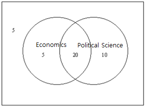
Since there are 25 students who take Economics and 20 students taking both courses, 25 - 20 = 5 students take only Economics. Also, since there are 30 students who take Political Science, 30 - 20 = 10 students take only Political Science. Thus, as shown in <Figure 5.2.1>, the number of students taking either Economics or Political Science is 5 + 10 + 20 = 35. Therefore, the probability of students taking either Economics or Political Science is 35 / 40.
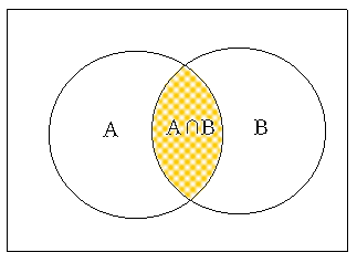
Consider the case of students taking both Economics (A) and Political Science (B). The event that a student takes both courses are denoted as A ∩ B and is called an intersection event of A and B (<Figure 5.2.2>).
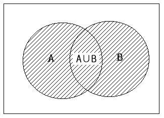
The event that a student takes either Economics or Political Science (one or both) is denoted as A ∪ B and is called an union event of A and B (<Figure 5.2.3>).
Probabilities of these events on this example are as follows:
P(B) = 30 / 40 = 0.750
P(A ∩ B) = 20 / 40 = 0.500
P(A ∪ B) = 35 / 40 = 0.875
The probability of P(A ∪ B) can also be calculated as follows if you look at the <Figure 5.2.1>.
That is, the probability of taking either Economics or Political Science, P(A ∪ B), can be calculated by adding the probability of taking each course and then by subtracting the probability of taking both courses.
[Addition Rule of Probability]
The rule discussed on [Example 5.2.3] is called the addition rule of probability.
$$\ P(A ∪ B) = P(A) + P(B) - P(A ∩ B) $$
If A ∩ B = ∅, then the rule becomes as follows:
$$ P(A ∪ B) = P(A) + P(B)$$
In this case, the events A and B are called mutually exclusive events.
Answer
In this case, because there are no students taking both courses, the events in which they take Economics (A) and Political Science (B) are mutually exclusive. Thus, the probability to take either Economics or Political Science, P(A U B), is as follows:
Let us consider the example below to find out the multiplication rule of probability.
Answer
To solve this problem, it is convenient to organize the information given into a cross table as shown below.
| Baku | Province | Total | |
|---|---|---|---|
| Male | 1 | 10 | |
| Female | 5 | 20 | |
| Total | 24 | 6 | 30 |
If we calculate and insert the blanks on the above table, it is as follows. Let us call the event of male as M, the female as F, from Baku as B, from the province as C.
| Baku(B) | Province(C) | Total | |
|---|---|---|---|
| Male(M) | 9 | 1 | 10 |
| Female(F) | 15 | 5 | 20 |
| Total | 24 | 6 | 30 |
1) \(\small P(C) = \) 6/30.
2) The probability that this student is from the province among females is 5/20. This probability is denoted as \(\small P(C∣F) \) and is called a conditional probability.
3) The probability of a male from the province is \(\small P(M∣C) = \) 1/6.
4) The probability is \(\small P(M ∩ B) \) and the cross table shows that the answer is 9/30. Alternatively, the probability of being a male among all students can be first obtained as \(\small P(M) = \) (10/30) and then multiplied by the conditional probability of being from Baku among males, \(\small P(B∣M) \) = 9/10. Namely
\( \qquad \small P(M ∩ B) = P(M) P(B∣M) = (10/30) \times (9/10) = 9/30 \)
This expression shows that the conditional probability \(\small P(B∣M) \) can be calculated by dividing \(\small P(M ∩ B) \) by \(\small P(M) \).
\( \qquad \small P(B ∣ M) = \frac {P(M ∩ B)} {P(M)} = \frac { 9/30} {10/30} = \frac {9} {10} \)
In addition, the probability \( \small P(M ∩ B) \) can be obtained first by the probability of being a student from Baku, \(\small P(B) = \) 24/30, and then multiplied by the probability of being a male from Baku (\(\small P(M∣B) = \) 9/24).
\( \qquad \small P(M ∩ B) = P(B) P(M∣B) = (24/30) × (9/24) \)
[Multiplication Rule of Probability]
You can calculate the conditional probabilities and their graphs using eStat as follows:
$$ \small P(A ∣ B) = \frac {P(A ∩ B)} {P(B)} \qquad \qquad \textrm{if} \quad P(B) ≠ 0 $$
In the above example, the probability of an intersection event is expressed by multiplying the probabilities of other events and it is called the multiplication rule of probability.
$$ \small P(A ∩ B) = P(A) P(B∣A) $$ If \(\small P(B∣A) = P(B) \), then the rule becomes as follows: $$ \small P(A ∩ B) = P(A) P(B) $$ In this case, the events \(\small A\) and \(\small B\) are called independent events.
Answer
Let us call the event that the Tiger wins the first game is \(\small A\) and the event that the Tiger wins the second game is \(\small B\). Since A and B are independent of each other, the probability that the Tiger is winning both games is as follows.
\( \qquad \small P(A ∩ B) = P(A) P(B) = 0.7 × 0.7 = 0.49 \)
| Baku(B) | Province(C) | Total | |
|---|---|---|---|
| Male(M) | 5 | 5 | 10 |
| Female(F) | 10 | 10 | 20 |
| Total | 15 | 15 | 30 |
Answer
Let us call the event of male as \(\small M \), female as \(\small F\), from Baku as \(\small B\), and from province as \(\small C \). From the table, probabilities of \(\small P(M ∩ B) \), \(\small P(M) \) and \(\small P(B) \) are as follows:
\( \qquad \small P(M ∩ B) = 5/30 \qquad P(M) = 10/30 \qquad P(B) = 15/30 \)
Therefore, the following relationship is satisfied:
\( \qquad \small P(M ∩ B) = P(M) P(B) \)
The events of male and Baku origin are independent of each other. Note that
\( \qquad \small P(M∣B) = 5/15 = 1/3 \qquad P(M)=10/30 \qquad \text{so, } \;\; P(M∣B) = P(M). \)
In this case, all events of both \(\small M \) and \(\small C \) , \(\small F \) and \(\small B \) , \(\small F \) and \(\small C \) are independent of each other. We call the two attributes, gender and region are independent of each other. In [Example 5.2.5], gender and region are not independent of each other.
The following is an example of how to calculate the probability of a complementary event.
Answer
The probability of finding one defective in the three product tests is as follows.
\( \qquad \small \frac { _4 C_2 \times _2 C_1 } {_6 C_3 } = \frac {3}{5}. \)
The probability of finding two defective products is as follows.
\( \qquad \small \frac { _4 C_1 \times _2 C_2 } {_6 C_3 } = \frac {1}{5}. \)
Thus, the probability that at least one defect will be found is 3/5 + 1/5 = 4/5. Another way to calculate this probability is to obtain the probability of an event in which there will be no defect (this is called a complementary event) and then, subtract it from 1. In other words, the probability that at least one defective product can be calculated as follows.
\( \qquad \small 1 - \frac { _4 C_3 } {_6 C_3 } = 1 - \frac {4}{20} = \frac {4}{5}. \)
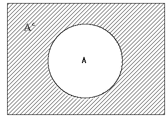
if \(\small A^C \) denotes a complementary event of the event \(\small A \), then \(\small P(A^C ) \) can be calculated as follows. $$ \small P(A^C) = 1 - P(A) $$
5.3 Discrete Random Variable
[presentation] [video]
In case of statistical experiments which are frequently observed around us, there are many similar probability calculations. For example, the problem of tossing coins several times to see how many times the head comes out is similar to counting how many defective products are made from a product line. This problem is also similar to counting the number of voters who support a particular candidate for the presidential election. In this section, the probability calculations as the previous examples, in general the discrete sample spaces are discussed.
Consider a statistical experiment in which a coin is thrown repeatedly two times. If the coin is ideal, the sample space for this experiment is {'Tail-Tail', 'Tail-Head', 'Head-Tail', 'Head-Head’}. The probability of an event in which each element of the sample space is produced is 1/4 by the classical definition. In most cases, the fact that we are interested in this example will be counting the number of heads or tails. If \(\small X\) is defined as 'the number of heads' in this experiment, the possible value of \(\small X\) can be 0, 1, or 2 and we are interested in calculating probabilities that \(\small X\)=0, \(\small X\)=1 or \(\small X\)=2. As such, a function that corresponds to one real number between [0,1] for each element of the sample space is called a random variable (see Table 5.3.1).
Table 5.3.1 Random variable \(\small X\) = 'Number of Heads’ when tossing a coin twice'
| Sample space | \(\small X\) = 'Number of Heads’ |
|---|---|
| Tail-Tail Tail-Head Head-Tail Head-Head |
0 1 1 2 |
Random variable is a function from the sample space to a real number.
When possible values of a random variable are finite or countably infinite, it is called a discrete random variable. If possible values of a random variable are uncountably infinite, it is called a continuous random variable.
Table 5.3.2 Probability distribution function of \(\small X\) = 'Number of Heads’ when tossing a coin twice'
| 1) Table style of the probability distribution function | 2) Function style of the probability distribution function | ||||
|---|---|---|---|---|---|
|
|
$$ \small \begin{align} f(x) &= 1/4, \qquad \text{if } x = 0 \\ &= 2/4, \qquad \text{if } x = 1 \\ &= 1/4, \qquad \text{if } x = 2 \\ \end{align} $$ |
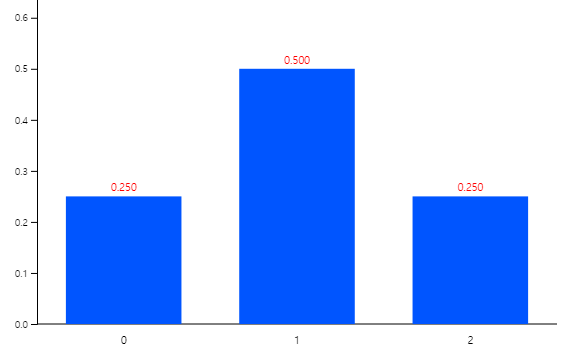
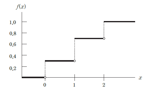
Table 5.3.3 Cumulative distribution function of the random variable \(\small X\) = 'Number of Heads’ when tossing a coin twice'
| 1) Table style of the cumulative distribution function | 2) Function style of the cumulative distribution function | ||||
|---|---|---|---|---|---|
|
|
$$ \begin{align} F(x) &= 0, \qquad\quad \text{if } x < 0 \\ &= 1/4, \qquad \text{if } 0 \le x < 1 \\ &= 3/4, \qquad \text{if } 1 \le x < 2 \\ &= 1, \qquad\quad \text{if } 2 \le x \end{align} $$ |
If probability for each value of the random variable \(X\) is summarized as a function, it is called a probability distribution function of \(X\) and usually denoted as f(x).
The cumulative probability of \(P(X \le x)\) as the value of random variable \(X\) increases is referred to as a cumulative distribution function and denoted as F(x).
| Hospital visit | 0 | 1 | 2 | 3 | 4 |
| Houshold | 74 | 80 | 30 | 10 | 6 |
Answer
1) Probability distribution function
| \(\small X = x\) | \(\small P(X = x)\) |
|---|---|
| 0 1 2 3 4 |
0.37 0.40 0.15 0.05 0.03 |
| Total | 1.00 |
2) Cumulative distribution function
| \(\small X = x\) | \(\small P(X \le x)\) |
|---|---|
| 0 1 2 3 4 |
0.37 0.77 0.92 0.97 1.00 |
If you select [Discrete Distribution] from 『eStatU』 menu, data input window appears as follows. Enter the data here as shown in the figure and click [Execute] button to display the probability distribution graph as in <Figure 5.3.3>.
[Discrete Distribution]
$$ \begin{align} E(X) &= \mu = \sum _{i=1} ^{n} x_{i} P(\textrm{X}= x_{i} ) \\ V(X) &= \sigma^2 = \sum_{i=1} ^{n} ( x_i - \mu )^2 P(\textrm{X}= x_i ) = \sum_{i=1}^{n} x_i ^2 P(\textrm{X}= x_i ) - \mu^2 \end{align} $$
Answer
Expectation and variance of \(\small X\) are as follows:
$$ \small \begin{align} E(X) &= \mu = \sum_{i=1}^{n} x_{i} \text{P(X } = x_{i} ) = 0 \times \frac{1}{4} + 1 \times \frac{2}{4} + 2 \times \frac{1}{4} = 1 \\ V(X) &= \sigma^2 = \sum_{i=1}^{n} x_{i}^{2} \textrm{ P(X} = x_{i} )- \mu^{2} = 0^{2} \times \frac{1}{4} + 1^{2} \times \frac{2}{4} + 2^{2} \times \frac{1}{4} - 1^{2} = \frac{1}{2} \end{align} $$
$$ \begin{align} E(aX + b) &= a E(X) + b \\ V(aX + b) &= a^2 V(X) \end{align} $$
Answer
The random variable \(\small X\) is the mid-term score and its mean and variance are \(\small E(X)\) = 60 and \(\small V(X)\) = 100.
1) The mean and variance of the new random variable \(\small X\) + 20 are as follows.
\(\qquad \small E(X + 20) = E(X) + 20 = 60 + 20 \) \(\qquad \small V(X + 20) = V(X) = 100\)
2) The mean and variance of the new random variable 1.4\(\small X\) are as follows.
\(\qquad \small E(1.4X) = 1.4 E(X) = 1.4 × 60 = 84\) \(\qquad \small V(1.4X) = 1.4^2 V(X) = 1.96 × 100 = 196 \)
3) The mean and variance of the new random variable 1.2X + 10 are as follows:
\(\qquad \small E(1.2X + 10) = 1.2 E(X) + 10 = 1.2 × 60 + 10 = 82 \) \(\qquad \small V(1.2X + 10) = 1.2^2 V(X) = 1.44 × 100 = 144 \)
If the mean of a random variable \(X\) is \mu, and the standard deviation is σ, then \(Z = \frac{X-\mu}{\sigma}\) is a new random variable with the mean of 0 and the variance of 1. This new random variable is referred to as a standardized random variable.
5.3.1 Binomial Distribution
[presentation] [video]
[Binomial Experiment]
Answer
This problem is the enforcement of Bernoulli trial in each game of 'win' and 'fail'. This Bernoulli trial is repeated four times. The sample space is all about winning or losing game and there are elements shown as follows by marking the winning in O and the losing in X.
S = {‘XXXX’, ‘OXXX’, ‘XOXX’, ‘XXOX’, ‘XXXO’, ‘OOXX’, ‘OXOX’, ‘OXXO’, ‘XOOX’, ‘XOXO’, ‘XXOO’, ‘OOOX’, ‘OOXO’, ‘OXOO’, ‘XOOO’, ‘OOOO’}
1) The event that the Tiger will lose all games is {'XXXX'} and the probability of this event is (0.4)×(0.4)×(0.4)×(0.4) = \(\small (0.4)^4\).
2) There are four events that the Tiger is winning once and losing three times such as {‘OXXX’, ‘XOXX’, ‘XXOX’, ‘XXXO’}. These four cases are equal to the number of O's in a single seat when there are four seats which is \(\small{}_4C_1\). Since the probability of each event is (0.6)×(0.4)×(0.4)×(0.4), the probability of the Tiger winning once is \(\small{}_4C_1 (0.6)(0.4)^3\).
3) There are six events that the Tiger is winning two times and losing two times such as {‘OOXX’, ‘OXOX’, ‘OXXO’, ‘XOOX’, ‘XOXO’, ‘XXOO’}. These six cases are equal to the number of O's in two seats when there are four seats which is \(\small{}_4C_2\). Since the probability of each event is (0.6)×(0.6)×(0.4)×(0.4), the probability of the Tiger winning twice is \(\small{}_4C_2 (0.6)^2(0.4)^2\).
4) There are four events that the Tiger is winning three times and losing one time such as {‘OOOX’, ‘OOXO’, ‘OXOO’, ‘XOOO’}. These four cases are equal to the number of O's in three seats when there are four seats which is \(\small{}_4C_3\). Since the probability of each event is (0.6)×(0.6)×(0.6)×(0.4), the probability of the Tiger winning three times is \(\small{}_4C_3 (0.6)^3(0.4)^1\).
5) There is one event that the Tiger is winning four times such as {‘OOOO’}. This one case is equal to the number of O's in four seats when there are four seats which is \(\small{}_4C_4\). Since the probability of each event is (0.6)×(0.6)×(0.6)×(0.6), the probability of the Tiger winning all four times is \(\small{}_4C_4 (0.6)^4\).
6) The probability distribution function of the random variable X = ‘the number of games the Tiger wins’ is a summary of the above probabilities.
| \(\small X = x \) | \(\small P(X=x) \) |
|---|---|
| 0 | \(\small {}_{4}C_0 (0.4)^4 = 0.0256 \) |
| 1 | \(\small {}_{4}C_1 (0.6) (0.4)^3 = 0.1536 \) |
| 2 | \(\small {}_{4}C_2 (0.6)^2 (0.4)^2 = 0.3456 \) |
| 3 | \(\small {}_{4}C_3 (0.6)^3 (0.4) = 0.3456 \) |
| 4 | \(\small {}_{4}C_4 (0.6)^4 = 0.1296 \) |
Answer
Select [Binomial Distribution] from the menu of 『eStatU』 and enter \(\small n = 4, p = 0.6\) and press the [Execute] button to display a binomial function graph as shown in <Figure 5.3.4>. Table 5.3.4 shows the table when you click the [Binomial Prob Table] button. This table makes it easy to obtain Binomial distribution probabilities from [Example 5.3.4].
[Binomial Distribution]
There are sliding bars of \(n\) and \(p\) and a probability calculation box under the graph, so put the desired value and press the [Enter] key to calculate the value.
To the right of the graph, a table of binomial distributions is shown. In addition to \(P(X = x)\), this table shows the cumulative probabilities \(P(X \le x)\) and \(P(X \ge x)\) to facilitate various probability calculations. If you select a new \(n\) and \(p\) and click [Execute] button, new binomial distribution table for this value is added below.
Table 5.3.4 『eStatU』 Binomial distribution table when \(\small n = 4, p = 0.6\)
| \(n = 4\) | \(p = 0.600\) | ||
|---|---|---|---|
| \(x\) | \(\small P(X = x)\) | \(\small P(X \le x)\) | \(\small P(X \ge x)\) |
| 0 | 0.0256 | 0.0256 | 1.0000 |
| 1 | 0.1536 | 0.1792 | 0.9744 |
| 2 | 0.3456 | 0.5248 | 0.8208 |
| 3 | 0.3456 | 0.8704 | 0.4752 |
| 4 | 0.1296 | 1.0000 | 0.1296 |
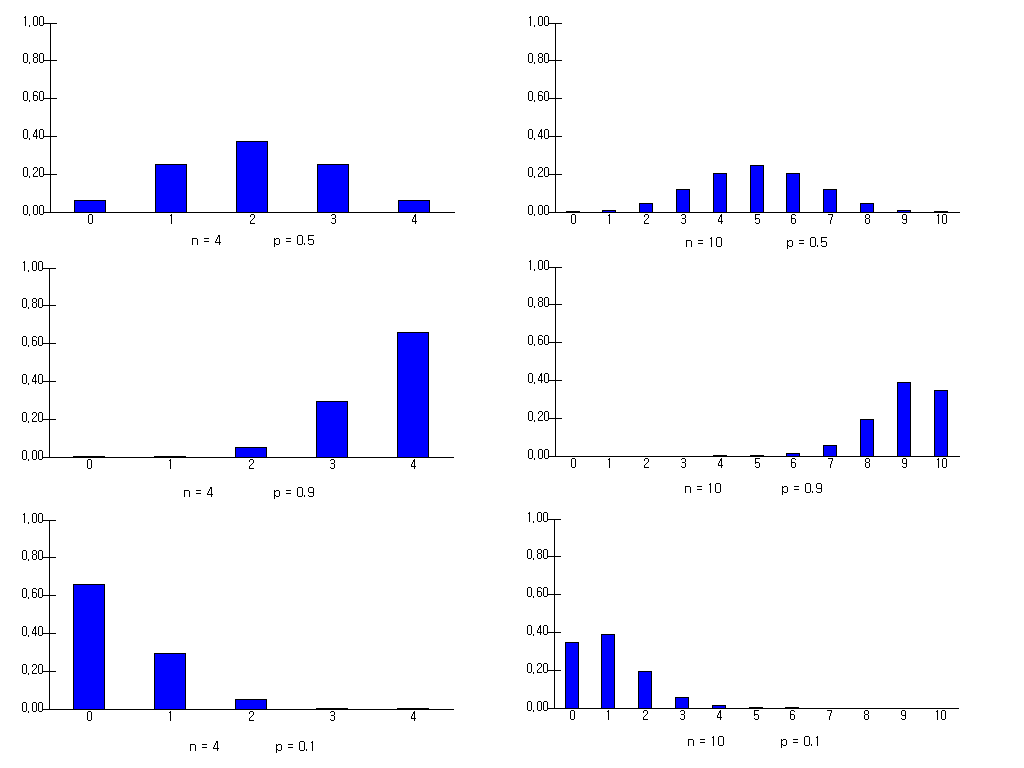
If the probability of success is \(p\) in a Bernoulli trial and the trial is repeated \(n\) times independently, the probability distribution function that the random variable \(X\) = the number of success’ is \(x\) is as follows: It is called a binomial distribution and denoted as \(B(n,p)\). $$ f(x) = {}_n C_x p^x (1-p)^{n-x} , \qquad x = 0,1,2, ... , n $$ The expectation and variance of the binomial distribution are as follows. $$ E(X) = np, V(X) = np(1-p) $$
Answer
This is a Binomial distribution with \(n = 10, p = 0.2\).
\( \qquad \quad \small P(X=3) = {}_{10} C_3 (0.2)^3 (1-0.2)^{10-3} = 0.2013 \)
$$ \small \begin{multline} \shoveleft P(X \ge 2) = 1 - P(X=0) - P(X=1) \\ \shoveleft = 1 - {}_{10} C_0 (0.2)^0 (1-0.2)^10 - {}_{10} C_1 (0.2)^1 (1-0.2)^10-1 = 1 - 0.1074 - 0.2684 = 0.6242\\ \end{multline} $$
\( \qquad \quad \small E(X) = np = 10 × 0.2 = 2 \)
\( \qquad \quad \small V(X) = np(1-p) = 10 × 0.2 × 0.8 = 1.6 \)
\( \qquad \quad \small \sigma(X) = 1.265 \)
Select ‘Binomial Distribution’ from the menu of 『eStatU』, enter \(n=10, p=0.2\), and click on the [Execute] button to display the graph shown in <Figure 5.3.6>. Checking 'Show Probability' option shows the probability on each bar where you can see the values in the above calculations.
Pressing the [Binary Prob Table] button will show the Binomial distribution table shown in Table 5.3.6. From here you can see that \(\small P(X \ge 2)\) = 0.6242
Table 5.3.5 『eStatU』 Binomial Distribution Table when \(n = 10, p = 0.2\)
| \(n = 10\) | \(p = 0.200\) | ||
|---|---|---|---|
| \(x\) | \(\small P(X = x)\) | \(\small P(X \le x)\) | \(\small P(X \ge x)\) |
| 0 | 0.1074 | 0.1074 | 1.0000 |
| 1 | 0.2684 | 0.3758 | 0.8926 |
| 2 | 0.3020 | 0.6778 | 0.6242 |
| 3 | 0.2013 | 0.8791 | 0.3222 |
| 4 | 0.0881 | 0.9672 | 0.1209 |
| 5 | 0.0264 | 0.9936 | 0.0328 |
| 6 | 0.0055 | 0.9991 | 0.0064 |
| 7 | 0.0008 | 0.9999 | 0.0009 |
| 8 | 0.0001 | 1.0000 | 0.0001 |
| 9 | 0.0000 | 1.0000 | 0.0000 |
| 10 | 0.0000 | 1.0000 | 0.0000 |
Answer
When you select \(n=50, p=0.05\) from the ‘Binomial Distribution’ of 『eStatU』 and click on the [Execute] button, the graph such as <Figure 5.3.7> appears. If you click the [Binomial Prob Table] button, then Table 5.3.6 appears.
1) You can check \(\small P(X=0)\) = 0.0769 easily from the table.
| \(n = 50\) | \(p = 0.050\) | ||
|---|---|---|---|
| \(x\) | \(\small P(X = x)\) | \(\small P(X \le x)\) | \(\small P(X \ge x)\) |
| 0 | 0.0769 | 0.0769 | 1.0000 |
| 1 | 0.2025 | 0.2794 | 0.9231 |
| 2 | 0.2611 | 0.5405 | 0.7206 |
| 3 | 0.2199 | 0.7604 | 0.4595 |
| 4 | 0.1360 | 0.8964 | 0.2396 |
| \(\cdots\) | \(\cdots\) | \(\cdots\) | \(\cdots\) |
\( \qquad \small P( 1 \le X \le 3) = P( X \le 3) - P( X \le 0) = 0.7604 – 0.0769 = 0.6835 \)
\( \qquad \small P(X \ge 3) = 1 - P( X \le 2) = 1 – 0.5405 = 0.4595 \)
5.3.2 Poisson Distribution
[presentation] [video]
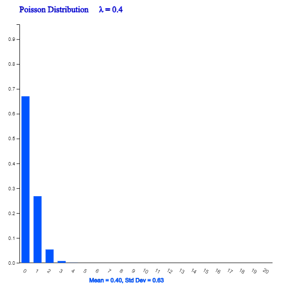
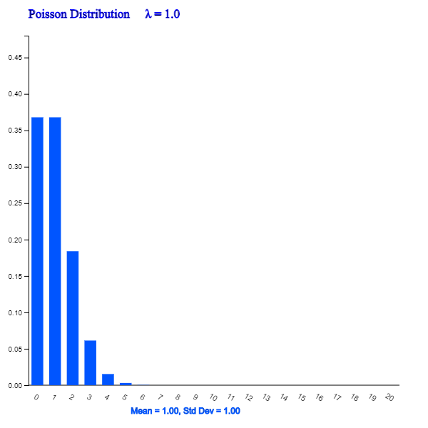
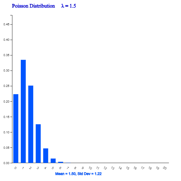
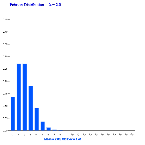
Probability of the Poisson distribution can be calculated using the following formula.
The distribution of a Poisson random variable \(X\) = 'Occurrence of success event per unit time or unit area' is as follows when the average number of success is λ. $$ f(x) = \frac { e^{-\lambda} \lambda^x } { x! } , \qquad x = 0, 1, 2, ... $$
The expectation and variance of the Poisson random variable are as follows. $$ E(X) = \lambda, \quad V(X) = \lambda $$
Answer
Let \(\small X\) be the Poisson random variable with λ = 5.
1) \(\small P(X = 0) = f(0) = \frac { e^{-5} {5}^{0} } { 0! } \) = 0.0067
2) \(\small P(X = 5) = f(5) = \frac { e^{-5} {5}^{5} } { 5! } \) = 0.1755
3) \(\small P(X \ge 2) = 1 - P(X \le 1) = 1 - P(X=0) - P(X=1) \) = 1 - 0.0067 - 0.0337 = 0.9596
Answer
Select [Poisson distribution] from the menu of 『eStatU』 and select λ = 2.5. Then click on the [Execute] button to display a graph such as <Figure 5.3.12> and click the [Poisson Prob Table] button to see the Table 5.3.7.
[Poisson Distribution]
| λ = 2.5 | |||
|---|---|---|---|
| \(x\) | \(\small P(X = x)\) | \(\small P(X \le x)\) | \(\small P(X \ge x)\) |
| 0 | 0.0821 | 0.0821 | 1.0000 |
| 1 | 0.2052 | 0.2873 | 0.9179 |
| 2 | 0.2565 | 0.5438 | 0.7127 |
| 3 | 0.2138 | 0.7576 | 0.4562 |
| 4 | 0.1336 | 0.8912 | 0.2424 |
| \(\cdots\) | \(\cdots\) | \(\cdots\) | \(\cdots\) |
1) \(\small P(X=1)\) = 0.2052.
2) \(\small P( 2 \le X \le 4)\) can be calculated as follows:
\(\qquad \small P( 2 \le X \le 4 ) = P( X \le 4) - P( X \le 1) \)= 0.8912 – 0.2873 = 0.6039
\(\qquad \small P(X \ge 2) = 1 - P( X \le 1) \)= 1 – 0.2873 = 0.7127
5.3.3 Geometric Distribution
[presentation] [video]
The probability of success \(p\) in the geometrical distribution is called a parameter of the geometric distribution. The probability distribution function of the geometric distribution is as follows:
When the probability of 'success' in a Bernoulli trial is \(p\) and \(X\) is the number of Bernoulli trials until the first success, the probability distribution of \(X\) is called a geometric distribution and its probability distribution function is as follows. $$ f(x) = (1-p)^{x-1} p, \qquad x=1,2, ... $$
The expectation and variance of the geometric random variable are as follows. $$ E(X) = \frac {1}{p}, \quad V(X) = \frac {1-p}{p^2 } $$
Answer
The probability of meeting opposed person is 0.4. Let \(\small X\) be the geometric random variable with \(p\) = 0.4.
1) \(\small P(X = 1) = f(1) = \small (1-0.4)^{1-1} 0.4 \) = 0.4
2) \(\small P(X = 5) = f(5) = \small (1-0.4)^{5-1} 0.4 \) = 0.0518
Answer
Select [Geometric Distribution] from the 『eStatU』 menu, select parameter \(p\) = 0.05, and click the [Execute] button to display the graph shown in <Figure 5.3.16>, and click the [Geometric Prob Table] button to display Table 5.3.8.
[Geometric Distribution]
| \(p\) = 0.05 | |||
|---|---|---|---|
| \(x\) | \(\small P(X = x)\) | \(\small P(X \le x)\) | \(\small P(X \ge x)\) |
| 1 | 0.0500 | 0.0500 | 1.0000 |
| 2 | 0.0475 | 0.0975 | 0.9500 |
| 3 | 0.0451 | 0.1426 | 0.9025 |
| 4 | 0.0429 | 0.1855 | 0.8574 |
| 5 | 0.0407 | 0.2262 | 0.8145 |
| \(\cdots\) | \(\cdots\) | \(\cdots\) | \(\cdots\) |
1) We can easily find \(\small P(X=3)\) = 0.0451.
2) We can easily find \(\small P(X \ge 3)\) = 0.9025.
\(\qquad \small P(X \ge 3) = 1 - P( X \le 2)\) = 1 – 0.0975 = 0.9025
5.3.4 Hypergeometric Distribution
[presentation] [video]
$$ \frac { { }_{15} C_2 \times {}_{5} C_1 } { {}_{20} C_3 } $$
Consider a population of size \(N\) which consists of \(D\) ‘success’ and \(N-D\) ‘failure’. If we collect a sample of size without replacement and \(X\) is the number of ‘success’ in the sample, then the distribution of \(X\) is called hypergeometric distribution and its probability distribution function is as follows. $$ \frac { {}_{D} C_x \times {}_{N-D} C_{n-x} } { {}_{N} C_{n} } $$ If we let \(p = \frac{D}{N}\), the expectation and variance of the hypergeometric random variable are as follows. $$ E(X) = np , \quad V(X) = np(1-p) \frac{N-n}{N-1} $$
Answer
These probability calculations have already been studied using combinations in section 5.1. This is the hypergeometric distribution with \(N\) = 20, \(D\) = 15, \(n\) = 3, so the probabilities are as follows.
$$ \small \begin{multline} \shoveleft P(X=1) = \frac { {}_{15} C_{2} \times {}_{5} C_{1} } {{}_{20} C_{3}} = \frac {15 \times 10} {1140} = 0.460 \\ \shoveleft P(X=2) = \frac { {}_{15} C_{1} \times {}_{5} C_{2} } {{}_{20} C_{3}} = \frac {105 \times 5} {1140} = 0.132 \\ \shoveleft P(X=3) = \frac { {}_{15} C_{0} \times {}_{5} C_{3} } {{}_{20} C_{3}} = \frac {455 \times 1} {1140} = 0.099 \\ \end{multline} $$
Answer
Select [Hypergeometric Distribution] from the menu of 『eStatU』, select \(N = 20, D = 15, n = 3 \) and click on the [Execute] button to display a graph such as <Figure 5.3.20>. If you click the [Hypergeometric Prob Table] button, Table 5.3.9 appears. This table shows the probabilities of \(\small P(X=0), P(X=1), P(X=2)\), and \(\small P(X=3)\).
[HyperGeometric Distribution]
| \(\small N = 20\) | \(\small D = 5 \) | \(\small n = 3 \) | |
|---|---|---|---|
| \(x\) | \(\small P(X = x)\) | \(\small P(X \le x)\) | \(\small P(X \ge x)\) |
| 0 | 0.3991 | 0.3991 | 1.0000 |
| 1 | 0.4605 | 0.8596 | 0.6009 |
| 2 | 0.1316 | 0.9912 | 0.1404 |
| 3 | 0.0088 | 1.0000 | 0.0088 |
5.4 Continuous Random Variable
[presentation] [video]
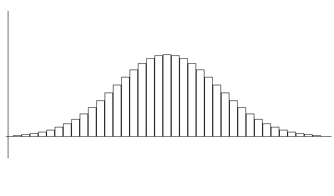
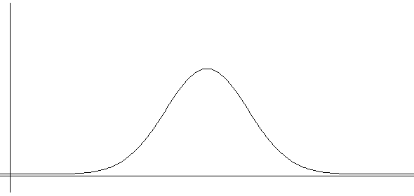
In case of the continuous random variable, calculating probability at each value of the random variable is meaningless, because there are infinite possible values and the probability at each value is considered zero. Instead of calculating the probability at a single value, the probability of an interval is of interest in case of the continuous random variable. For example, 'What is the probability of a commuting time between 25 and 35 minutes?' In order to obtain this probability, we can divide the sample space of the commuting time into several intervals and count the number of their frequencies and probabilities for 100 days as in Table 5.4.1. <Figure 5.4.1> is a histogram of this table.
Table 5.4.1 Frequency table of the commuting time for 100 days \(\small X\) = ‘commuting time’ (unit: minute)
| Interval \((a \le X \lt b)\) | Frequency | Probability |
|---|---|---|
| \( 10 \le X \lt 30 \) \( 30 \le X \lt 50 \) \( 50 \le X \lt 60 \) \( 60 \le X \lt 70 \) \( 70 \le X \lt 90 \) |
5 30 40 20 5 |
5/100 30/100 40/100 20/100 5/100 |
| Total | 100 (days) | 1 |
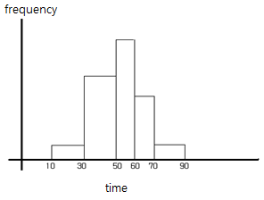
$$ P(30 \le X \lt 60) = 30/100 + 40/100 = 70/100 $$

Answer
Since the random variable \(\small X\) has the same possibility as any number between 10 and 30, the probability distribution function (uniform distribution) is as follows.
\( \quad \small f(x) = \Big\{ \array { \frac {1}{30-10}, &\quad \text{if 10 < }x \text { < 30} \cr 0, &\qquad \text{elsewhere} } \)
<Figure 5.4.5> is the shape of this probability distribution function and it is called a uniform distribution between 10 and 30 denoted as Uniform(10,30).
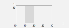
The probability of the delivery time between 15 and 20 minutes is the area of the shaded rectangle of the <Figure 5.4.5> which can be calculated as follows.
\( \quad \small P(15 \lt X \lt 20) = (20 - 15) × \frac {1}{20} = 0.25 \)
5.4.1 Normal Distribution
[presentation] [video]
[Normal Experiment]
A normal distribution function or a Gaussian distribution function is as follows. $$ f(x) = \frac{1}{\sqrt{2 π} \, \sigma } exp \{ - \frac {(x-\mu)^2 } {2 \sigma^2} \} $$ This distribution function has two parameters μ and σ, each representing the mean and standard deviation of the normal distribution.
[ ]
The following graph shows three-normal distributions \(N(-3, 1)\), \(N(0, 1)\) and \(N(3, 1)\) in which the mean is different from each other and the variance is all 1. If the mean is different, the graph of the same shape is moved horizontally.
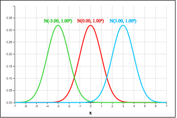
Comparison of three graphs of normal distribution, \(N(-3, 1)\), \(N(0, 1)\), \(N(3, 1)\)
|
The following graph shows three-normal distributions \(N(0, 0.5^2 )\), \(N(0, 1)\) and \(N(0, 3^2 )\) in which all means are zero and variances are different. It can be observed that all of them are symmetrical around the average 0, and that the normal distribution becomes flat as the variance increases, and the normal distribution becomes sharp as the variance decreases.
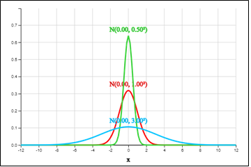
Comparison of three graphs of normal distribution, \(N(0, 0.5^2 )\), \(N(0, 1)\), \(N(0, 3^2 )\)
|
Probability Calculation of the Normal Distribution
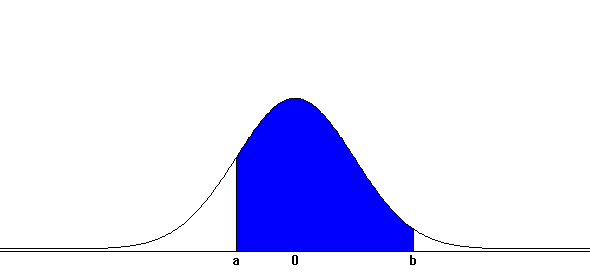
Mathematically, this area must be obtained with the following definite integral over \( (a,b) \), but it is impossible to calculate by hand and can only be calculated using a computer. $$ P(a \lt X \lt b)= \int_{a} ^{b} {} \frac{1}{\sqrt{2 π} \, \sigma } exp \{ - \frac {(x-\mu)^2 } {2 \sigma^2} \}dx $$ If X is a normal random variable with the mean μ and variance \(\sigma^2\), a standardized random variable \(Z = \frac {X - \mu}{\sigma} \) is a normal random variable with the mean 0 and variance 1, i.e., \(Z ∼ N(0,1)\). This fact implies that, if we can find probabilities of all types of intervals in N(0,1) distribution, then we can also find probabilities of all types of intervals in \(N(\mu, \sigma^2 )\). Therefore, \(N(0,1)\) is called a standard normal distribution or simply \(\small Z\) distribution.
If \(X\) is a normal random variable with the mean μ and variance \(\sigma^2\), i.e. \(X ∼ N(\mu,\sigma^2) \), then the standardized random variable \(Z\), \( \frac{X-\mu}{\sigma} \) follows a Normal distribution with the mean 0 and variance 1, i.e. \( Z ∼ N(0,1) \)
|
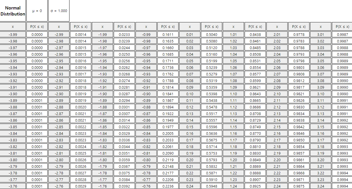
Table 5.4.2 Standard normal distribution table by using 『eStatU』
|
In 『eStatU』, the calculation of probability \( P( a \lt X \lt b ) \) for the interval \((a , b)\) of any normal distribution \( N(\mu,\sigma^2) \) can be done as in <Figure 5.4.9>, and the percentile \(x\) for a given probability \(p\), which is \(P( X \lt x) = p\), can also be easily calculated. In 『eStatU』, the probability of any interval on [μ - 4σ, μ + 4σ ] can be calculated.
[Normal Distribution]
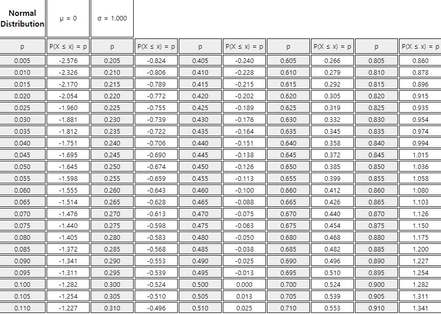
The probability of \(P(Z \lt z)\) is near 0 if z is less than μ - 4σ and is 1 if z is greater than μ + 4σ. Table 5.4.3 shows percentiles of the standard normal distribution by using 『eStatU』.
1) \(\small P(Z \lt 1.96)\)
2) \(\small P(-1.96 \lt Z \lt 1.96)\)
3) \(\small P(Z \gt 1.96)\)
Answer
By using standard normal distribution table,
1) \(\small P(Z \lt 1.96)\) = 0.975.
2) \(\small P(-1.96 \lt Z \lt 1.96) = P(Z \lt 1.96) - P(Z \lt -1.96)\) = 0.975 - 0.025 = 0.95
3) \(\small P(Z \gt 1.96) = 1 - P(Z \lt 1.96)\) = 1 - 0.975 = 0.025
By using normal distribution module of 『eStatU』 (<Figure 5.4.9>),
Answer
By using percentile table of the standard normal distribution,
By using normal distribution module of 『eStatU』 (<Figure 5.4.9>),
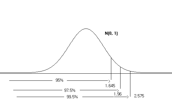
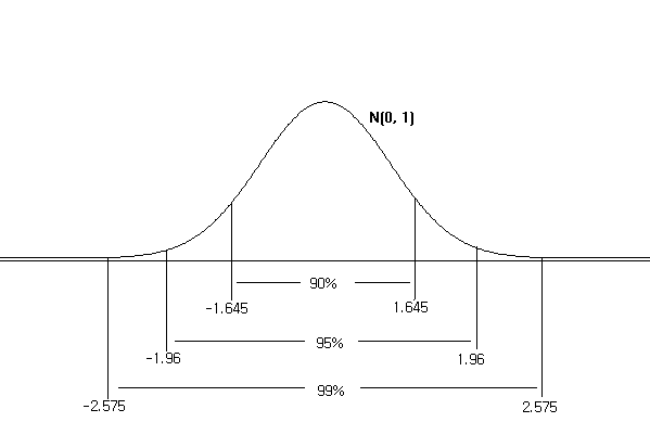
i.e., \(P(-1.96 \lt Z \lt 1.96)\) = 0.95, \(P(-2.575 \lt Z \lt 2.575)\) = 0.99
When \(X\) is a normal random variable with a mean μ and variance \(\sigma^2\), \(Z = \frac{X-\mu}{\sigma}\) follows the standard normal distribution. Therefore, the probability \(P( a \lt X \lt b ) \) of the interval \( (a,b) \) of \(X\) is as follows: $$ P( a \lt X \lt b ) = P( \frac {a - \mu}{\sigma} \lt Z \lt \frac {b - \mu}{\sigma} ) $$
1) \(\small P(X \lt 94.3) \)
2) \(\small P(X \gt 57.7) \)
3) \(\small P(57.7 \lt X \lt 94.3) \)
Answer
By using transformation to the standardized normal random variable, probability calculations are as follows:
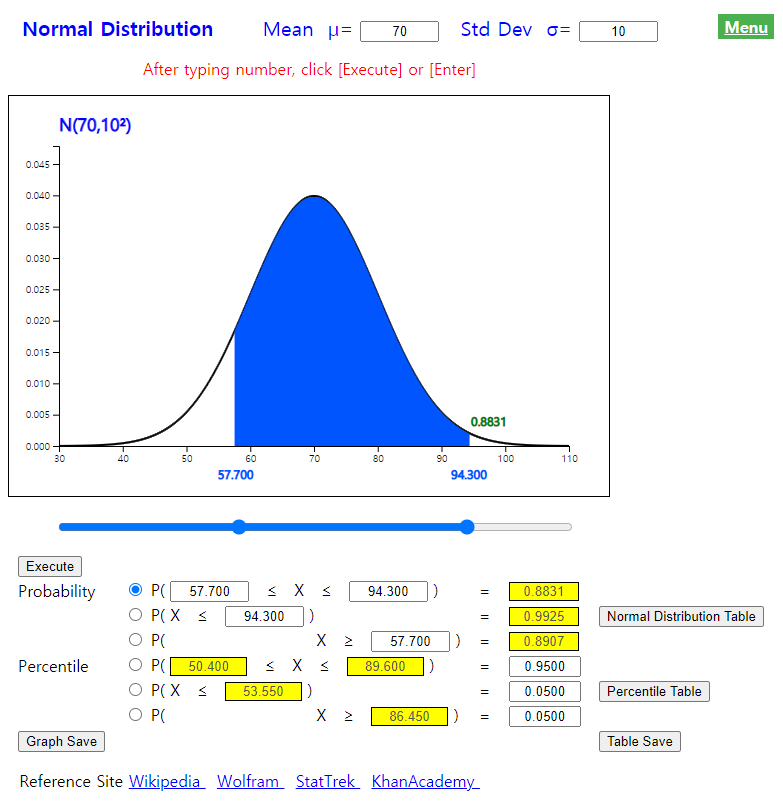
1) \(\small P (X \lt 94.3) = P( \frac {X - 70}{10} \lt \frac {94.3 - 70}{10} ) = P( Z \lt 2.43) = 0.9925 \)
2) \(\small P (X \gt 57.7) = P( \frac {X - 70}{10} \gt \frac {57.7 - 70}{10} ) = P( Z \gt -1.23 = 0.8907\)
3) \(\small P (57.7 \lt X \lt 94.3) = P( \frac {57.7 - 70}{10} \lt \frac {X - 70}{10} \lt \frac {94.3 - 70}{10} ) = P(-1.23 \lt Z \lt 2.43 ) = 0.8832 \)
By using 『eStatU』, to obtain a probability of the normal distribution , enter the mean as 70 and the standard deviation as 10 at the top of the screen as <Figure 5.4.12>.
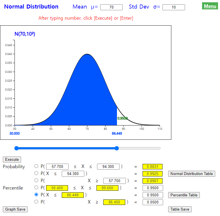
1) What is the 95% percentile of the mid-term test scores?
2) What is the 95% percentile of two-sided type of the mid-term scores?
Answer
By using normal probability table, percentile calculations are as follows:
By using 『eStatU』, to obtain the probability of normal distribution , enter the mean as 70 and the standard deviation as 10 at the top of the screen as <Figure 5.4.13>.
Normal Approximation of Binomial Distribution
Answer
If the number of defective products is \(\small X\), \(\small X\) is a binomial distribution with \(n = 100, p = 0.05\). When \(n\) is this large, we calculate the probability approximately using normal distribution. Since the mean of this binomial distribution is \(np\) = 100 × 0.05 = 5, and the variance is \(np(1-p)\) = 100 × 0.05 x (1-0.05) = 4.75, we use the normal distribution \(\small N(5, 4.75)\) to calculate the probability approximately as follows.
1) \( \small P( X \lt 2) = P( Z \lt \frac{2-5}{\sqrt{4.75}} ) = P(Z \lt -1.376) = 0.0845 \)
2) \( \small P( 3 \lt X \lt 7) = P( \frac{3-5}{\sqrt{4.75}} \lt Z \lt \frac{7-5}{\sqrt{4.75}} ) = P( -0.918 \lt Z \lt 0.918) = 0.642 \)
5.4.2 Exponential Distribution
[presentation] [video]
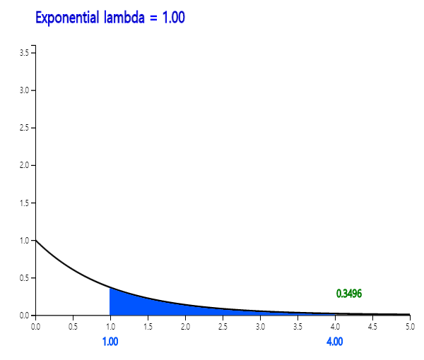
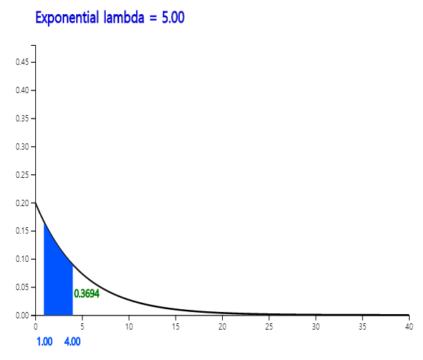
These examples appear when events occur at the same rate at a given time (e.g., three calls per hour, etc.). If the average number of events per unit hour is λ and \(\small X\) is the random variable of the time between events, then \(\small X\) is an exponential random variable. λ is a parameter of the exponential distribution and the formula for the exponential probability distribution function is as follows:
When the average number of events per unit hour is λ and the random variable \(X\) is the time between events, the probability distribution function of \(X\) is as follows.
$$ f(x) = \lambda \, exp(-\lambda x ), \qquad x \gt 0 $$ It is called an exponential distribution and its expectation and variance are as follows. $$ E(X) = \frac{1}{\lambda } , \quad V(X) = \frac{1}{\lambda^2} $$
Example 5.4.7 If the life span of a product has the average of 10 hours and follows an exponential distribution, obtain the following probabilities using 『eStatU』.
Answer
In 『eStatU』, select [Exponential Distribution] and enter λ = 10. Click the [Execute] button to reveal the graph shown as <Figure 5.4.16>.
[Exponential Distribution]
