The group variable used to distinguish groups of the population, such as the grade or the rice, is called a factor.
In testing hypothesis of the population mean described in chapters 7 and 8, the number of populations was one or two. However, many cases are encountered where there are three or more population means to compare. The analysis of variance (ANOVA) is used to test whether several population means are equal or not. The ANOVA was first published by British statistician R. A. Fisher as a test method applied to the study of agriculture, but today its principles are applied in many experimental sciences, including economics, business administration, psychology and medicine.
In section 9.1, the one-way ANOVA for single factor is introduced. In section 9.2, experimental designs for experiments are introduced. In section 9.3, the two-way ANOVA for two factors experiments is introduced.
The group variable used to distinguish groups of the population, such as the grade or the rice, is called a factor.
The group variable used to distinguish groups of the population is called a factor.
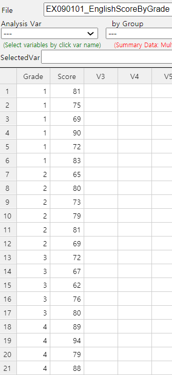
Example 9.1.1 In order to compare the English proficiency of each grade at a university, samples were randomly selected from each grade to take the same English test, and data are as in Table 9.1.1. The last row is a calculation of the average \({\overline y}_{1\cdot}\), \({\overline y}_{2\cdot}\), \({\overline y}_{3\cdot}\), \({\overline y}_{4\cdot}\) for each grade.
| Socre | Student 1 | Student 2 | Student 3 | Student 4 | Student 5 | Student 6 | Student Average |
|---|---|---|---|---|---|---|---|
| Grade 1 | 81 | 75 | 69 | 90 | 72 | 83 | \({\overline y}_{1\cdot}\)=78.3 |
| Grade 2 | 65 | 80 | 73 | 79 | 81 | 69 | \({\overline y}_{2\cdot}\)=74.5 |
| Grade 3 | 72 | 67 | 62 | 76 | 80 | \({\overline y}_{3\cdot}\)=71.4 | |
| Grade 4 | 89 | 94 | 79 | 88 | \({\overline y}_{4\cdot}\)=87.5 |
[Ex] ⇨ eBook ⇨ EX090101_EnglishScoreByGrade.csv.
Answer

However, this treatment sum of squares can be larger if the number of populations increases. It requires modification to become a test statistic to determine whether several population means are equal. The squared distance from each observation to its sample mean of the grade is called the within sum of squares (SSW) or the error sum of squares (SSE) as defined below.
If population distributions of English scores in each grade follow normal distributions and their variances are the same, the following test statistic has the \(F_{3, 17}\) distribution.
This statistic can be used to test whether population English scores of four grades are the same or not. In the test statistic, the numerator \(\frac{SSTr}{4-1}\) is called the treatment mean square (MSTr) which implies a variance between grade means. The denominator \(\frac{SSE}{21-4}\) is called the error mean square (MSE) which implies a variance within each grade. Thus, the above test statistics are based on the ratio of two variances which is why the test of multiple population means is called an analysis of variance (ANOVA).
Calculated test statistic which is the observed \(\small F\) value, \(\small F_{0}\) , using data of English scores for each grade is as follows.
Since \(\small F_{3,17; 0.05}\) = 3.20, the null hypothesis that population means of English scores of each grade are the same, \(\small H_0 : \mu_1 = \mu_2 = \mu_3 = \mu_4 \) , is rejected at the 5% significance level. In other words, there is a difference in population means of English scores of each grade.
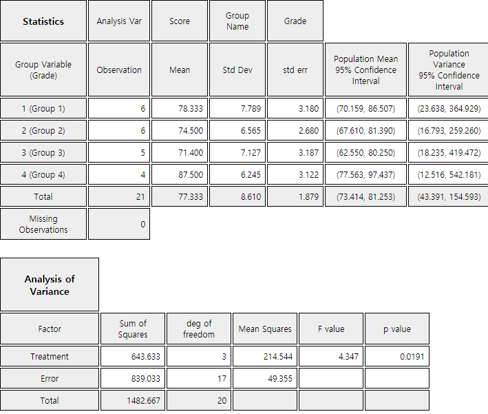
The following ANOVA table provides a single view of the above calculation.
| Factor | Sum of Squares | Degree of freedom | Mean Squares | F ratio |
|---|---|---|---|---|
| Treatment | SSTr = 643.633 | 4-1 | MSTr = \(\frac{643.633}{3}\) | \(F_0 = 4.347\) |
| Error | SSE = 839.033 | 21-4 | MSE = \(\frac{839.033}{17}\) | |
| Total | SST = 1482.666 | 20 |
The analysis of variance is also possible using 『eStatU』. Entering the data as in <Figure 9.1.7>
and clicking the [Execute] button will have the same result as in <Figure 9.1.5>.
[Testing Hypothesis : 3+ Population Means (ANOVA)]
The analysis of variance method that examines the effect of single factor on the response variable is called the one-way ANOVA. Table 9.1.2 shows the typical data structure of the one-way ANOVA when the number of levels of a factor is \(k\) and the numbers of observation at each level are \(n_1 , n_2 , ... , n_k\).
| Factor | Observed values of sample | Average |
|---|---|---|
| Level 1 | \(Y_{11} \; Y_{12}\; \cdots \;Y_{1n_1} \) | \(\overline Y_{1\cdot}\) |
| Level 2 | \(Y_{21} \; Y_{22}\; \cdots \;Y_{2n_2} \) | \(\overline Y_{2\cdot}\) |
| \(\cdots\) | \(\cdots\) | \(\cdots\) |
| Level k | \(Y_{k1} \; Y_{k2}\; \cdots \;Y_{kn_k} \) | \(\overline Y_{k\cdot}\) |
The error term \(\epsilon_{ij}\) is a random variable in the response variable due to reasons other than levels of the factor. For example, in the English score example, differences in English performance for each grade can be caused by other variables besides the variables of grade, such as individual study hours, gender and IQ. However, by assuming that these variations are relatively small compared to variations due to differences in grade, the error term can be interpreted as the sum of these various reasons.
The hypothesis to test can be represented using \(\alpha_{i}\) instead of \(\mu_{i}\) as follows:
In order to test the hypothesis, the analysis of variance table as Table 9.1.3 is used.
| Factor | Sum of Squares | Degree of freedom | Mean Squares | F ratio |
|---|---|---|---|---|
| Treatment | SSTr | \(k-1\) | MSTr=\(\frac{SSTr}{k-1}\) | \(F_0 = \frac{MSTr}{MSE}\) |
| Error | SSE | \(n-k\) | MSE=\(\frac{SSE}{n-k}\) | |
| Total | SST | \(n-1\) |
Sum of squares: SST = SSTr + SSE
Degrees of freedom: \((n-1) = (k-1) + (n-k)\)
The calculated \(F\) value, \(F_0\), in the last column of the ANOVA table represents the relative size of MSTr and MSE. If the assumptions of \(\epsilon_{ij}\) based on statistical theory are satisfied, and if the null hypothesis \(\small H_0 : \alpha_1 = \alpha_2 = \cdots = \alpha_k \) = 0 is true, then the below test statistic follows a F distribution with degrees of freedoms \(k-1\) and \(n-k\). $$ F_{0} = \frac { \frac{SSTr}{(k-1)} } { \frac{SSE}{(n-k)} } $$ Therefore, when the significance level is \(\alpha\) for a test, if the calculated value \(F_0\) is greater than the value of \(F_{k-1,n-k; α}\), then the null hypothesis is rejected. That is, it is determined that the population means of each factor level are not all the same.
(Note: 『eStat』 calculates the \(p\)-value of this test. Hence if the \(p\)-value is smaller than the significance level \(\alpha\), then reject the null hypothesis. )
The analysis of differences between population means after ANOVA requires several tests for the mean difference to be performed simultaneously and it is called as the multiple comparisons. The hypothesis for the multiple comparison to test whether the level means, \(\mu_i\) and \(\mu_j\), are equal is as follows: $$ H_0 : \mu_i = \mu_j , \quad H_1 : \mu_i \ne \mu_j \quad i=1,2,...,k-1,\; j=i+1,i+2,...,k $$ It means that there are \(_{k}C_{2}\) tests to be done simultaneously for the multiple comparisons if there are \(k\) levels of the factor.
There are many multiple comparisons tests, but Tukey's Honestly Significant Difference (HSD) test is most commonly
used. The statistic for Tukey's HSD test to compare means \(\mu_i\) and \(\mu_j\) is the sample mean
difference \({\overline y}_{i \cdot} - {\overline y}_{j \cdot}\) and the decision rule to test \(H_0 : \mu_i = \mu_j\) is as follows:
\(\qquad\)If \(|{\overline y}_{i\cdot} - {\overline y}_{j\cdot} | > HSD_{ij}\), then reject \(H_0\)
where \(HSD_{ij} = q_{k,n-k; α} \cdot \sqrt{\frac{1}{2} ( \frac{1}{n_i } + \frac{1}{n_j} ) MSE }\),
\(n_i\) and \(n_j\) are the number of samples (repetitions) in \(i^{th}\) level and \(j^{th}\) level,
\(MSE\) is the mean squared error, \(q_{k,n-k; α}\) is the right tail 100\(\times \alpha\)
percentile of the studentized range distribution with parameter \(k\) and \(n-k\) degrees of freedom.
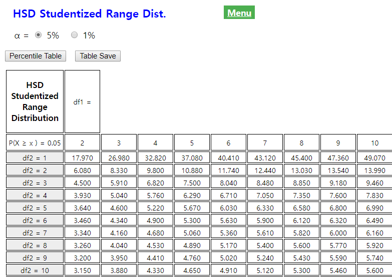
(It can be found at 『eStatU』 (<Figure 9.1.8>).
Example 9.1.2 In [Example 9.1.1], the analysis variance of English scores by the grade concluded that the null hypothesis was rejected and the average English scores for each grade were not all the same. Now let's apply the multiple comparisons to check where the differences exist among each school grade with the significance level of 5%. Use 『eStat』 to check the result.
Answer
The hypothesis of the multiple comparisons is \(\small H_0 : \mu_i = \mu_j , \quad H_1 : \mu_i \ne \mu_j\) and the decision rule is as follows:
Since there are four school grades (\(k=4\)), \(_{4}C_{2}\) = 6 multiple comparisons are possible as follows. The 5 percentile from the right tail of HSD distribution which is used to test is \(q_{k,n-k; α} = q_{4,21-4; 0.05}\) = 4.02.
1) \(\small H_0 : \mu_1 = \mu_2 , \quad H_1 : \mu_1 \ne \mu_2\)
2) \(\small H_0 : \mu_1 = \mu_3 , \quad H_1 : \mu_1 \ne \mu_3\)
3) \(\small H_0 : \mu_1 = \mu_4 , \quad H_1 : \mu_1 \ne \mu_4\)
4) \(\small H_0 : \mu_2 = \mu_3 , \quad H_1 : \mu_2 \ne \mu_3\)
5) \(\small H_0 : \mu_2 = \mu_4 , \quad H_1 : \mu_2 \ne \mu_4\)
6) \(\small H_0 : \mu_3 = \mu_4 , \quad H_1 : \mu_3 \ne \mu_4\)
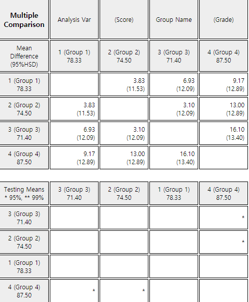
The result of the above multiple comparisons shows that there is a difference between \(\mu_2\) and \(\mu_4\), \(\mu_3\) and \(\mu_4\) as can be seen in the dot graph with average in <Figure 9.1.1>. It also shows that \(\mu_1\) has no significant difference from other means.
If you click [Multiple Comparison] in the options of the ANOVA as in <Figure 9.1.3>, 『eStat』 shows the result of Tukey's multiple comparisons as shown in <Figure 9.1.9>. 『eStat』 also shows the mean difference and 95% HSD value for the sample mean combination after rearranging levels of rows and columns in ascending order of the sample means.
The next table shows that, if the HSD test result for the combination of the two levels is significant with the 5% significance level, then * will be marked and if it is significant with the 1% significance level, then ** will be marked, if it is not significant, then the cell is left blank.
For the analysis of mean differences, confidence intervals for each level may also be used. <Figure 9.1.2> shows the 95% confidence interval for the mean for each level. This confidence interval is created using the formula described in Chapter 6, but the only difference is that the estimate of the variance for the error, \(\sigma^2\), is the pooled variance using overall observations rather than the sample variance of observed values at each level. In the ANOVA table, MSE is the pooled variance.
In post-analysis using these confidence intervals, there is a difference between means if the confidence intervals are not overlapped, so the same conclusion can be obtained as in the previous HSD test.
apply the multiple comparisons to check where differences exist among Control and two treatments with the significance level of 5%. Use 『eStat』.
Example 9.1.3 In [Example 9.1.1] of English score comparison by the grade, apply the residual analysis using 『eStat』.
Answer
If you click on [Standardized Residual Plot] of the ANOVA option in <Figure 9.1.3>, a scatter plot of residuals versus fitted values appears as shown in <Figure 9.1.10>. In this scatter plot, if the residuals show no unusual tendency around zero and appear randomly, then the assumptions of independence and homoscedasticity are valid. There is no unusual tendency in this scatter plot. Normality of the residuals can be checked by drawing the histogram of residuals.
apply the residual analysis using 『eStat』.
If five drivers (1, 2, 3, 4, 5) plan to drive the car to measure the fuel mileage of all cars a day, the fuel mileage of the car may be affected by the driver. One solution would be to allocate 15 cars randomly to five drivers and then to randomize the sequence of experiments as well. For example, each car is numbered from 1 to 15 and then, the experiment of the fuel mileage is conducted in the order of numbers that come out using drawing a random number. Such an experiment would reduce the likelihood of differences caused by external factors such as the driver, daily wind speed and wind direction, because randomized experiments make all external factors equally affecting the all observed measurement values. This method of experiments is called a completely randomized design of experiments. Table 9.2.1 shows an example allocation of experiments by this method. Symbols A, B and C represent the three types of cars.
| Driver | 1 | 2 | 3 | 4 | 5 |
|---|---|---|---|---|---|
| Car Type | B | A | B | C | A |
| B | C | A | A | C | |
| C | B | A | B | C |
In general, in order to achieve the purpose of the analysis of variance, it is necessary to plan experiments thoroughly in advance for obtaining data properly. The completely randomized design method explained as above is studied in detail at the Design of Experiments area in Statistics. From the standpoint of the experimental design, the one-way analysis of variance technique is called an analysis of the single factor design.
| Driver | 1 | 2 | 3 | 4 | 5 |
|---|---|---|---|---|---|
| Car Type | A(22.4) | B(12.6) | C(18.7) | A(21.1) | A(24.5) |
| (gas mileage) | C(20.2) | C(15.2) | A(19.7) | B(17.8) | C(23.8) |
| B(16.3) | A(16.1) | B(15.9) | C(18.9) | B(21.0) |
Table 9.2.2 shows that the total observed values are divided into five groups by driver, called blocks so that they have the same characteristics. The variable representing blocks, such as the driver, is referred to as a block variable. A block variable is considered generally if experimental results are influenced significantly by this variable which is different from the factor. For example, when examining the yield resulting from rice variety, if the fields of the rice paddy used in the experiment do not have the same fertility, divide the fields into several blocks which have the same fertility and then all varieties of rice are planted in each block of the rice paddy. This would eliminate the influence of the rice paddy which have different fertility and would allow for a more accurate examination of the differences in yield between rice varieties.
Statistical model of the randomized block design with \(b\) blocks can be represented as follows:
$$
Y_{ij} = \mu + \alpha_i + B_j + \epsilon_{ij}, \quad i=1,2, ... ,k, \; j=1,2, ... ,b
$$
In this equation, \(B_j\) is the effect of \(j^{th}\) level of the block variable to the response variable. In the randomized
block design, the variation resulting from the difference between levels of the block variable can be separated
from the error term of the variation of the factor independently. In the randomized block design, the total
variation is divided into as follows:
$$
Y_{ij} - {\overline Y}_{\cdot \cdot} = (Y_{ij} - {\overline Y}_{i \cdot} - {\overline Y}_{\cdot j} + {\overline Y}_{\cdot \cdot}) + ({\overline Y}_{i \cdot} - {\overline Y}_{\cdot \cdot}) +({\overline Y}_{\cdot j} - {\overline Y}_{\cdot \cdot})
$$
If you square both sides of the equation above and then combine for all \(i\) and \(j\), you can obtain
several sums of squares as in the one-way analysis of variance as follows:
Total sum of squares :
\(\qquad\)SST = \(\sum_{i=1}^{k} \sum_{j=1}^{b} ( Y_{ij} - {\overline Y}_{\cdot \cdot} )^2 \) ,
degrees of freedom ; \(bk - 1\)
Error sum of squares :
\(\qquad\)SSE = \(\sum_{i=1}^{k} \sum_{j=1}^{b} ( {Y}_{ij} - {\overline Y}_{i \cdot} - {\overline Y}_{\cdot j} + {\overline Y}_{\cdot \cdot})^2 \) ,
degrees of freedom ; \((b-1)(k-1)\)
Treatment sum of squares :
\(\qquad\)SSTr = \(\sum_{i=1}^{k} \sum_{j=1}^{b} ( {\overline Y}_{i \cdot} - {\overline Y}_{\cdot \cdot} )^2 \)
= \(b\sum_{i=1}^{k} ( {\overline Y}_{i \cdot} - {\overline Y}_{\cdot \cdot} )^2 \) ,
degrees of freedom ; \(k - 1\)
Block sum of squares :
\(\qquad\)SSB = \(\sum_{i=1}^{k} \sum_{j=1}^{b} ( {\overline Y}_{\cdot j} - {\overline Y}_{\cdot \cdot} )^2 \)
= \(k \sum_{j=1}^{b} ( {\overline Y}_{\cdot j} - {\overline Y}_{\cdot \cdot} )^2 \),
degrees of freedom ; \(b - 1\)
The following facts are always established in the randomized block design.
| Variation | Sum of Squares | Degree of freedom | Mean Squares | F value |
|---|---|---|---|---|
| Treatment | SSTr | \(k-1\) | MSTr=\(\frac{SSTr}{k-1}\) | \(F_0 = \frac{MSTr}{MSE}\) |
| Block | SSB | \(b-1\) | MSB=\(\frac{SSB}{b-1}\) | |
| Error | SSE | \((b-1)(k-1)\) | MSE=\(\frac{SSE}{(b-1)(k-1)}\) | |
| Total | SST | \(bk-1\) |
Example 9.2.1 Table 9.2.4 is the rearrangement of the fuel mileage data in Table 9.2.2 measured by five drivers and car types.
| Driver | 1 | 2 | 3 | 4 | 5 | Average(\(\overline y_{i \cdot}\)) |
|---|---|---|---|---|---|---|
| Car Type A | 22.4 | 16.1 | 19.7 | 21.1 | 24.5 | 20.76 |
| Car Type B | 16.3 | 12.6 | 15.9 | 17.8 | 21.0 | 16.72 |
| Car Type C | 20.2 | 15.2 | 18.7 | 18.9 | 23.8 | 19.36 |
| Average(\(\overline y_{\cdot j}\)) | 19.63 | 14.63 | 18.10 | 19.27 | 23.10 | 18.947 |
Answer
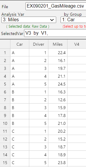
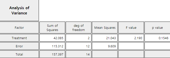
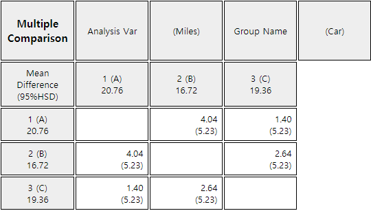
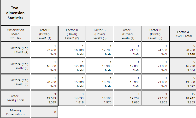
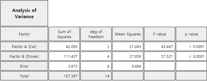
In average, car type A has the best fuel mileage than other car types. In order to examine more about the differences between car types, the multiple comparison test in the previous section can be applied. In this example, you can use one HSD value for all mean comparisons, because the number of repetitions (r) at each level is the same.
\(\quad \small HSD = q_{3,8; 0.05} \sqrt {\frac{MSE}{r}} = (4.041) \sqrt{\frac{0.484}{5}} \) = 1.257
Therefore, there is a significant difference in fuel mileage between all three types of cars, since the differences between the mean values (4.04, 1.40, 2.64) are all greater than the critical value of 1.257.
The same analysis of randomized design can be done using 『eStatU』 by following data input and clicking [Execute] button..
[ - ]
| Area 1 | Area 2 | Area 3 | |
|---|---|---|---|
| Wheat Type A | 50 | 60 | 56 |
| Wheat Type B | 59 | 52 | 51 |
| Wheat Type C | 55 | 55 | 52 |
| Wheat Type D | 58 | 58 | 55 |
In the Latin square design, we assign one sources of extraneous variation to the columns of the square and the second source of extraneous variation to the rows of the square. We then assign the treatments in such a way that each treatment occurs one and only once in each row and each column. The number of rows, the number of columns, and the number of treatments, therefore, are all equal.
Table 9.2.5 shows a 3 × 3 typical Latin squares with three rows, three columns and three treatments designated by capital letters A, B, C.
| Column 1 (Road 1) | Column 2 (Road 2 | Column 3 (Road 3) | |
|---|---|---|---|
| Row 1 (Driver 1) | A | B | C |
| Row 2 (Driver 2) | B | C | A |
| Row 3 (Driver 3) | C | A | B |
Table 9.2.6 shows a 4 × 4 typical Latin squares with four rows, four columns and four treatments designated by capital letters A, B, C, D.
| Column 1 (Road 1) | Column 2 (Road 2) | Column 3 (Road 3) | Column 4 (Road 4) | |
|---|---|---|---|---|
| Row 1 (Driver 1) | A | B | C | D |
| Row 2 (Driver 2) | B | C | D | A |
| Row 3 (Driver 3) | C | D | A | B |
| Row 4 (Driver 4) | D | A | B | C |
In the Latin square design, treatments can be assigned randomly in such a way that the car type occurs one and only once in each row and each column. Therefore, there are many possible designs of 3 × 3 and 4 × 4 Latin square. We get randomization in the Latin square by randomly selection a square of the desired dimension from all possible squares of that dimension. One method of doing this is to randomly assign a different treatments to each cell in each column, with the restriction that each treatment must appear one and only once in each row.
Small Latin squares provided only a small number of degrees of freedom for the error mean square. So a minimum size of 5 × 5 is usually recommended.
The hypothesis of Latin square design with \(r\) treatments is as follows:
Null Hypothesis \(\qquad \quad H_{0} : \mu_{1} = \mu_{2} = \cdots = \mu_{r} \)
Alternative Hypothesis \(\;\;\quad \; H_{1} : \) At least one pair of \(\mu_i \) is not equal.
Statistical model of the \(r × r \) Latin square design with \(r\) treatments can be represented as follows: $$ Y_{ijk} = \mu + \alpha_i + \beta_j + \gamma_k + \epsilon_{ijk}, \quad i=1,2, ... ,r, \; j=1,2, ... ,r, \; k=1,2, ... , r $$ Here \(\mu_i = \mu + \alpha_i\). In this equation, \(\alpha_i\) is the effect of \(i^{th}\) level of the row block variable to the response variable and \(\beta_j\) is the effect of \(j^{th}\) level of the column block variable to the response variable. \(\gamma_k\) is the effect of \(k^{th}\) level of the response variable.
Notation for row averages, column averages and treatment averages of \(r × r \) Latin squre data are as follows;
| Column 1 | Column 2 | \(\cdots \) | Column r | Row Average | |
|---|---|---|---|---|---|
| Row 1 | \({\overline Y}_{ 1 \cdot \cdot} \) | ||||
| Row 2 | \({\overline Y}_{ 2 \cdot \cdot} \) | ||||
| \(\cdots \) | \(\cdots \) | \(Y_{ijk}\) | \(\cdots \) | \(\cdots \) | |
| Row r | \({\overline Y}_{ r \cdot \cdot} \) | ||||
| Column Average | \({\overline Y}_{ \cdot 1 \cdot} \) | \({\overline Y}_{ \cdot 2 \cdot} \) | \(\cdots\) | \({\overline Y}_{ \cdot r \cdot} \) | \({\overline Y}_{ \cdot \cdot \cdot} \) |
| Treatment Average | \({\overline Y}_{ \cdot \cdot 1} \) | \({\overline Y}_{ \cdot \cdot 2} \) | \(\cdots\) | \({\overline Y}_{ \cdot \cdot r} \) |
In the Latin square design, the variation resulting from the difference between levels of two block variables can be separated from the error term of the variation of the factor independently. In the Latin square design, the total variation is divided into as follows:
$$
Y_{ijk} - {\overline Y}_{\cdot \cdot \cdot} = (Y_{ijk} - {\overline Y}_{i \cdot \cdot} - {\overline Y}_{\cdot j \cdot} - {\overline Y}_{\cdot \cdot k} + 2 {\overline Y}_{\cdot \cdot \cdot}) + ({\overline Y}_{i \cdot \cdot} - {\overline Y}_{\cdot \cdot \cdot}) + ({\overline Y}_{\cdot j \cdot} - {\overline Y}_{\cdot \cdot \cdot}) + ({\overline Y}_{\cdot \cdot k} - {\overline Y}_{\cdot \cdot \cdot})
$$
If you square both sides of the equation above and then combine for all \(i , j\) and \(k\), you can obtain
the following sums of squares:
Total sum of squares :
SST = \(\sum_{i=1}^{r} \sum_{j=1}^{r} \sum_{k=1}^{r} ( Y_{ijk} - {\overline Y}_{\cdot \cdot \cdot} )^2 \) ,
degrees of freedom ; \(r^2 - 1\)
Error sum of squares :
SSE = \(\sum_{i=1}^{r} \sum_{j=1}^{r} \sum_{k=1}^{r} ( {Y}_{ijk} - {\overline Y}_{i \cdot \cdot} - {\overline Y}_{\cdot j \cdot} - {\overline Y}_{\cdot \cdot k} + 2 {\overline Y}_{\cdot \cdot \cdot})^2 \) ,
degrees of freedom ; \((r-1)(r-2)\)
Row sum of squares :
SSR = \(\sum_{i=1}^{r} \sum_{j=1}^{r} \sum_{k=1}^{r} ( {\overline Y}_{i \cdot \cdot} - {\overline Y}_{\cdot \cdot \cdot} )^2 \)
degrees of freedom ; \(r - 1\)
Column sum of squares :
SSC = \(\sum_{i=1}^{r} \sum_{j=1}^{r} \sum_{k=1}^{r} ( {\overline Y}_{\cdot j \cdot} - {\overline Y}_{\cdot \cdot \cdot} )^2 \)
degrees of freedom ; \(r - 1\)
Treatment sum of squares :
SSTr = \(\sum_{i=1}^{r} \sum_{j=1}^{r} \sum_{k=1}^{r} ( {\overline Y}_{\cdot \cdot k} - {\overline Y}_{\cdot \cdot \cdot} )^2 \)
degrees of freedom ; \(r - 1\)
The following facts are always established in the Latin square design.
Sum of squares : SST = SSE + SSR + SSC + SSTr
Degrees of freedom : \(r^2 -1 = (r-1)(r-2) + (r-1) + (r-1) + (r-1) \)
| Variation | Sum of Squares | Degree of freedom | Mean Squares | F value |
|---|---|---|---|---|
| Treatment | SSTr | \(r-1\) | MSTr=\(\frac{SSTr}{r-1}\) | \(F_0 = \frac{MSTr}{MSE}\) |
| Row | SSR | \(r-1\) | MSR=\(\frac{SSB}{r-1}\) | |
| Columnk | SSC | \(r-1\) | MSC=\(\frac{SSB}{r-1}\) | |
| Error | SSE | \((r-1)(r-2)\) | MSE=\(\frac{SSE}{(r-1)(r-2))}\) | |
| Total | SST | \(r^2 -1\) |
Example 9.2.2 Table 9.2.9 is the fuel mileage data of four car types (A, B, C, D) measured by four drivers and four road types with Latin square design.
| Column 1 (Road 1) | Column 2 (Road 2) | Column 3 (Road 3) | Column 4 (Road 4) | |
|---|---|---|---|---|
| Row 1 (Driver 1) | A (22) | B (16) | C (19) | D (21) |
| Row 2 (Driver 2) | B (24) | C (16) | D (12) | A (15) |
| Row 3 (Driver 3) | C (17) | D (21) | A (20) | B (15) |
| Row 4 (Driver 4) | D (18) | A (18) | B (23) | C (22) |
Use 『eStatU』 to do the analysis of variance whether the four car types have the same fuel mileage.
Answer
In 『eStatU』, click [Testing Hypothesis ANOVA – Latin Square Design], select the number of treatment r = 4 and enter data as shown in <Figure 9.2.10>.
Click [Execute] button to show Dot graph by car type in Latin square design as <Figure 9.2.11> and ANOVA table as in <Figure 9.2.12>. The dot graph and result of the ANOVA is that there is no difference in fuel mileage between the car types.
[ - ]
| Time of week | Column 1 (Day 1) | Column 2 (Day 2 | Column 3 (Day 3) | Column 4 (Day 4) |
|---|---|---|---|---|
| Row 1 (Store 1) | A | B | C | D |
| Row 2 (Store 2) | B | C | D | A |
| Row 3 (Store 3) | C | D | A | B |
| Row 4 (Store 4) | D | A | B | C |
When data are obtained from repeated experiments at each factor level, the two-way ANOVA tests whether the population means of each level of factor A are the same (called the main effect test of the factor A) as the one-way ANOVA, or tests whether the population means of each level of factor B are the same (called the main effect test of the factor B). In addition, the two-way ANOVA tests whether the effect of one factor A is influenced by each level of the other factor B (called the interaction effect test). For example, in a chemical process, if the higher the pressure when the temperature is low, the greater the amount of products, and the lower the pressure when the temperature is high, the greater the amount of products, the interaction effect exists between the two factors of temperature and pressure. The interaction effect exists where the effects of one factor change with changes in the level of another factor.
When data are obtained from repeated experiments at each factor level, the two-way ANOVA tests whether the population means of each level of factor A (called the main effect test of the factor A) are the same as the one-way ANOVA, or tests whether the population means of each level of factor B are the same (called the main effect test of the factor B).
The two-way ANOVA also tests whether the effect of one factor A is influenced by each level of the other factor B (called the interaction effect test).
Example 9.3.1 Table 9.3.1 shows the yield data of three repeated agricultural experiments for each combination of four fertilizer levels and three rice types to investigate the yield of rice.
| Fertilizer | Rice type 1 | Rice type 2 | Rice type 3 |
|---|---|---|---|
| 1 | 64, 66, 70 | 72, 81, 64 | 74, 51, 65 |
| 2 | 65, 63, 58 | 57, 43, 52 | 47, 58, 67 |
| 3 | 59, 68, 65 | 66, 71, 59 | 58, 45, 42 |
| 4 | 58, 50, 49 | 57, 61, 53 | 53, 59, 38 |
Answer
| (Factor B) Fertilizer |
(Factor A) Rice type 1 |
(Factor A) Rice type 2 |
(Factor A) Rice type 3 |
Row Average |
|---|---|---|---|---|
| 1 | \(\overline y_{11\cdot}\) = 66.7 | \(\overline y_{12\cdot}\) = 72.3 | \(\overline y_{13\cdot}\) = 63.3 | \(\overline y_{1\cdot\cdot}\) = 67.4 |
| 2 | \(\overline y_{21\cdot}\) = 62.0 | \(\overline y_{22\cdot}\) = 50.7 | \(\overline y_{23\cdot}\) = 57.3 | \(\overline y_{2\cdot\cdot}\) = 56.7 |
| 3 | \(\overline y_{31\cdot}\) = 64.0 | \(\overline y_{32\cdot}\) = 65.3 | \(\overline y_{33\cdot}\) = 48.3 | \(\overline y_{3\cdot\cdot}\) = 59.2 |
| 4 | \(\overline y_{41\cdot}\) = 52.3 | \(\overline y_{42\cdot}\) = 57.0 | \(\overline y_{43\cdot}\) = 50.0 | \(\overline y_{4\cdot\cdot}\) = 53.1 |
| Column Average | \(\overline y_{\cdot1\cdot}\) = 61.3 | \(\overline y_{\cdot2\cdot}\) = 61.3 | \(\overline y_{\cdot3\cdot}\) = 54.8 | \(\overline y_{\cdot\cdot\cdot}\) = 59.1 |
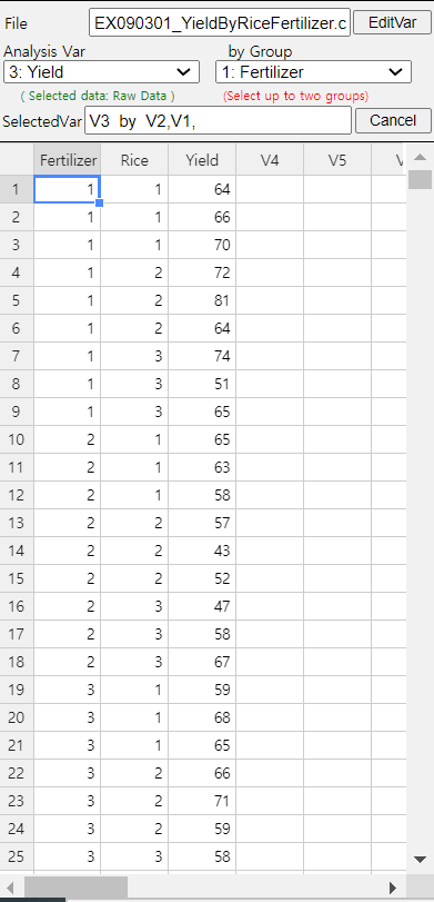
If the null hypothesis is rejected, we conclude that the main effect of rice types exists. In order to test the main effect of rice types, as in the one-way analysis of variance, the sum of squared distances from each average yield \({\overline y}_{\cdot j \cdot}\) of rice type to the overall average yield \({\overline y}_{\cdot \cdot \cdot}\).
\(\quad \small {SSA} = 12(61.3-{\overline y}_{\cdot \cdot \cdot})^2 + 12(61.3-{\overline y}_{\cdot \cdot \cdot})^2 + 12(54.8-{\overline y}_{\cdot \cdot \cdot})^2 \) = 342.39
where the weight of 12 of each sum of squares is calculated by the number of data for each rice type. Since there are 3 rice types, the degrees of freedom of \(\small SSA\) is (3-1) and we call the sum of squares \(\small SSA\) divided by (3-1), \(\frac{SSA}{(3-1)}\), is the mean squares of factor A, \(\small MSA\).
Testing the factor B, which is to test the main effect of fertilizer types, implies to test the following null hypothesis.
\(\quad \small H_0\) : The average yields of the four fertilizer types are the same.
If the null hypothesis is rejected, we conclude that the main effect of fertilizer types exists. In order to test the main effect of fertilizer types, as in the one-way analysis of variance, the sum of squared distances from each average yield \({\overline y}_{i \cdot \cdot}\) of fertilizer type \(i\) to the overall average yield \({\overline y}_{\cdot \cdot \cdot}\),
\(\quad \small {SSB} = 9(67.4 - {\overline y}_{\cdot \cdot \cdot})^2 + 9(56.7 - {\overline y}_{\cdot \cdot \cdot} )^2 + 9(59.2 - {\overline y}_{\cdot \cdot \cdot})^2 + 9(53.1 - {\overline y}_{\cdot \cdot \cdot})^2 \) = 1002.89
where the weight of 9 of each sum of squares is calculated by the number of data for each fertilizer type. Since there are 4 fertilizer types, the degrees of freedom of \(\small SSB\) is (4-1) and we call the sum of squares \(\small SSB\) divided by (4-1), \(\frac{SSB}{(4-1)}\), is the mean squares of factor B, \(\small MSB\).
Testing the interaction effect of rice and fertilizer (represented as factor AB) is to test the following null hypothesis.
\(\quad \small H_0\) : There is no interaction effect between rice type and fertilizer type.
If the null hypothesis is rejected, we conclude that there is an interaction effect between rice types and fertilizer types. In order to test the interaction effect, the sum of squared distances from each average yield \({\overline y}_{ij \cdot}\) subtracting the average yield \({\overline y}_{i \cdot \cdot}\) of fertilizer type \(i\), subtracting the average yield \({\overline y}_{\cdot j \cdot}\) of rice type \(j\), adding the overall average yield \({\overline y}_{\cdot \cdot \cdot}\).
\(\quad\) \(\small {SSAB} = 3(66.7- {\overline y}_{1 \cdot \cdot} - {\overline y}_{\cdot 1 \cdot} +{\overline y}_{\cdot \cdot \cdot})^2 + 3(72.3- {\overline y}_{1 \cdot \cdot} -{\overline y}_{\cdot 2 \cdot} +{\overline y}_{\cdot \cdot \cdot})^2 + 3(63.3- {\overline y}_{1 \cdot \cdot} - {\overline y}_{\cdot 3 \cdot} +{\overline y}_{\cdot \cdot \cdot})^2 \)
\(\qquad\) \(\small + 3(62.0- {\overline y}_{2 \cdot \cdot} - {\overline y}_{\cdot 1 \cdot} +{\overline y}_{\cdot \cdot \cdot})^2 + 3(50.7- {\overline y}_{2 \cdot \cdot} - {\overline y}_{\cdot 2 \cdot} +{\overline y}_{\cdot \cdot \cdot})^2 + 3(57.3- {\overline y}_{2 \cdot \cdot} -{\overline y}_{\cdot 3 \cdot} +{\overline y}_{\cdot \cdot \cdot})^2 \)
\(\qquad\) \(\small + 3(64.0- {\overline y}_{3 \cdot \cdot} - {\overline y}_{\cdot 1 \cdot} +{\overline y}_{\cdot \cdot \cdot})^2 + 3(65.3- {\overline y}_{3 \cdot \cdot} - {\overline y}_{\cdot 2 \cdot} +{\overline y}_{\cdot \cdot \cdot})^2 + 3(48.3- {\overline y}_{3 \cdot \cdot} - {\overline y}_{\cdot 3 \cdot} +{\overline y}_{\cdot \cdot \cdot})^2 \)
\(\qquad\) \(\small + 3(52.3- {\overline y}_{4 \cdot \cdot} - {\overline y}_{\cdot 1 \cdot} +{\overline y}_{\cdot \cdot \cdot})^2 + 3(57.0- {\overline y}_{4 \cdot \cdot} - {\overline y}_{\cdot 2 \cdot} +{\overline y}_{\cdot \cdot \cdot})^2 + 3(50.0- {\overline y}_{4 \cdot \cdot} -{\overline y}_{\cdot 3 \cdot} +{\overline y}_{\cdot \cdot \cdot})^2 \)
where the weight of 3 of each sum of squares is calculated by the number of data for each cell of rice and fertilizer type. The degrees of freedom of \(\small SSAB\) is (3-1)(4-1) and we call the sum of squares \(\small SSAB\) divided by (3-1)(4-1), \(\small \frac {SSAB}{(3-1)(4-1)}\) is the mean squares of interaction AB, \(\small MSAB\).
It is not possible to test each effect immediately using these sum of squares, but the error sum of squares should be calculated. In order to calculate the error sum of squares, first we calculate the total sum of squares which is the sum of the squared distances from each data to the overall average.
\(\quad \small {SST} = ( 64 -{\overline y}_{\cdot \cdot \cdot})^2 + ( 66 -{\overline y}_{\cdot \cdot \cdot})^2 + ( 70 -{\overline y}_{\cdot \cdot \cdot})^2 + \cdots + ( 53 -{\overline y}_{\cdot \cdot \cdot})^2 + ( 59 -{\overline y}_{\cdot \cdot \cdot})^2 + ( 38 -{\overline y}_{\cdot \cdot \cdot})^2 = 3267.56 \)
This total sum of squares can be proven mathematically to be the sum of the other sums of squares as follows:
\(\quad \small {SST} = SSA + SSB + SSAB + SSE \)
Therefore, the error sum of squares can be calculated as follows:
\(\quad \small {SSE} = SST - (SSA + SSB + SSAB) \)
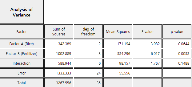
If the yields on each rice type or fertilizer type are assumed to be normal and the variances are the same, the statistic which divides the each mean squares by the error mean squares follows \(F\) distribution. Therefore, the main effects and interaction effect can be tested using \(F\) distributions. If the interaction effect is separated, we test them first. Testing results using the 5% significance level are as follows:
① Testing of the interaction effect on rice and fertilizer:
\(\qquad \small F_0 = \frac {MSAB}{MSE} = \frac { \frac{SSAB}{(3-1)(4-1)} } {\frac {SSE}{24}} \) = 1.77
\(\qquad \small F_{6,24; 0.05} \) = 2.51
② Testing of the main effect on rice types (Factor A):
\(\qquad \small F_0 = \frac {MSA}{MSE} = \frac { \frac{SSA}{(3-1)} } {\frac {SSE}{24}} \) = 3.08
\(\qquad \small F_{2,24; 0.05} \) = 3.40
③ Testing of the main effect on fertilizer types (Factor B):
\(\qquad \small F_0 = \frac {MSB}{MSE} = \frac { \frac{SSB}{(4-1)} } {\frac {SSE}{24}} \) = 6.02
\(\qquad \small F_{3,24; 0.05} \) = 3.01
The result of the two-way analysis of variances is as Table 9.3.3.
| Factor | Sum of Squares | Degree of freedom | Mean Squares | F value | p value |
|---|---|---|---|---|---|
| Rice Type | 342.3889 | 2 | 171.1944 | 3.0815 | 0.0644 |
| Fertilizer Type | 1002.8889 | 3 | 334.2963 | 6.0173 | 0.0033 |
| Interaction | 588.9444 | 6 | 98.1574 | 1.7668 | 0.1488 |
| Error | 1333.3333 | 24 | 55.5556 | ||
| Total | 3267.5556 | 35 |
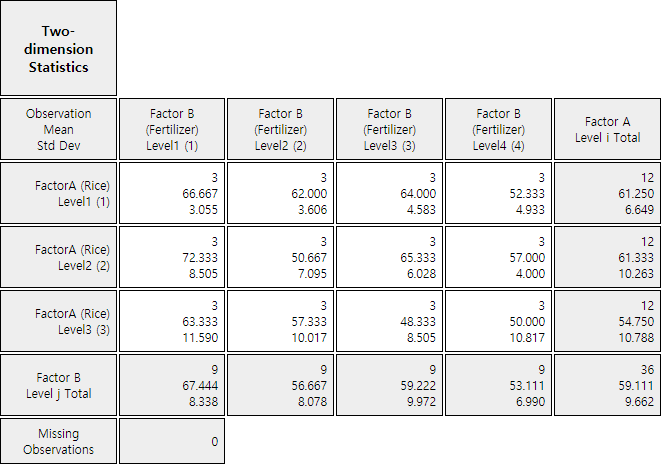
The same analysis of two factors ANOVA can be done using 『eStatU』 by following data input and clicking [Execute] button..
[]
Sum of Squares: \(\qquad SST = SSA + SSB + SSAB + SSE\)
degrees of freedom: \((n-1) = (a-1) + (b-1) + (a-1)(b-1) + (n-ab)\)
| Factor | Sum of Squares | Degree of freedom | Mean Squares | F value |
|---|---|---|---|---|
| Factor A | SSA | \(a-1\) | MSA=\(\frac{SSA}{a-1}\) | \(F_1 = \frac{MSA}{MSE}\) |
| Factor B | SSB | \(b-1\) | MSB=\(\frac{SSB}{b-1}\) | \(F_2 = \frac{MSB}{MSE}\) |
| Interaction | SSAB | \((a-1)(b-1)\) | MSAB=\(\frac{SSAB}{(a-1)(b-1)}\) | \(F_3 = \frac{MSAB}{MSE}\) |
| Error | SSE | \(n-ab\) | MSE=\(\frac{SSE}{(n-ab)}\) | |
| Total | SST | \(n-1\) |
If there is no repeated observation at each level combination of two factors, the interaction effect can not be estimated and the row of interaction factor is deleted from the above two-way ANOVA table. In this case, the analysis of variance table is the same as the randomized block design as Table 9.2.3.
1) Test for the interaction effect:
\(\quad\)\(H_0 : \gamma_{ij} = 0,\; i=1,2,...,a;\; j=1,2,...,b \)
\(\qquad\quad \)If \(\frac{MSAB}{MSE} \gt F_{(a-1)(b-1),n-ab; α} \), then reject \(H_0\)
2) Test for the main effect of factor A:
\(\quad\)\(H_0 : \alpha_1 = \alpha_2 = \cdots = \alpha_a = 0 \)
\(\qquad\quad\)If \(\frac{MSA}{MSE} \gt F_{(a-1),n-ab; α} \), then reject \(H_0\)
3) Test for the main effect of factor B:
\(\quad\)\(H_0 : \beta_1 = \beta_2 = \cdots = \beta_b = 0 \)
\(\qquad\quad\)If \(\frac{MSB}{MSE} \gt F_{(b-1),n-ab; α} \), then reject \(H_0\)
(『eStat』 calculates the \(p\)-value for each of these tests and tests them using it. That is,
for each test, if the \(p\)-value is less than the significance level, the null hypothesis
\(H_0\) is rejected.)
If the test for interaction effect is not significant, a test of the main effects of each factor can be performed to test significant differences between levels. However, if there is a significant interaction effect, the test for the main effects of each factor is meaningless, so an analysis should be made on which level combinations of factors show differences in the means.
If you conclude that significant differences between the levels of a factor as in the one-way analysis of variance exist there, you can compare confidence intervals at each level to see which level of the differences appears. And a residual analysis is necessary to investigate the validity of the assumption.
| (Unit: Time) | Humidity \(H_1\) | Humidity \(H_2\) |
|---|---|---|
| Time \(T_1\) | 6.29 6.38 6.25 |
5.95 6.05 5.89 |
| Time \(T_2\) | 5.80 5.92 5.78 |
6.32 6.44 6.29 |
Even in the two-way analysis of variance, obtaining sample data at each level of two factors in engineering or in agriculture can be influenced by other factors and should be careful in sampling. In order to accurately identify the differences that may exist between each level of a factor, it is advisable to make as few as possible influences from other factors. One of the most commonly used methods of doing this is completely randomized design which makes the entire experiments random. There are many other experimental design methods, and for more information, refer to the references to the experimental design of several factors.